注意:本篇为50天后的Java自学笔记扩充,内容不再是基础数据结构内容而是机器学习中的各种经典算法。这部分博客更侧重与笔记以方便自己的理解,自我知识的输出明显减少,若有错误欢迎指正!
目录

一、算法概念
这部分内容在老师的博客中已经讲得非常完备,因此本篇博客更像是我自己学习笔记的追踪和同步。
首先是有下面这样的数据集(下载:https://gitee.com/fansmale/javasampledata):
@relation weather.symbolic

@attribute outlook {sunny, overcast, rainy}
@attribute temperature {hot, mild, cool}
@attribute humidity {high, normal}
@attribute windy {TRUE, FALSE}
@attribute play {yes, no}

@data
sunny,hot,high,FALSE,no
sunny,hot,high,TRUE,no
overcast,hot,high,FALSE,yes
rainy,mild,high,FALSE,yes
rainy,cool,normal,FALSE,yes
rainy,cool,normal,TRUE,no
overcast,cool,normal,TRUE,yes
sunny,mild,high,FALSE,no
sunny,cool,normal,FALSE,yes
rainy,mild,normal,FALSE,yes
sunny,mild,normal,TRUE,yes
overcast,mild,high,TRUE,yes
overcast,hot,normal,FALSE,yes
rainy,mild,high,TRUE,no
这里的每列数据都构成了一个类别属性,这就是我们所在意的符号型数据(无实际值特性的枚举数据类)。这里前四个为一般的描述天气现状的数据,而最后一列的{Yes, No}则描述了一个决断,即根据四个天气的描述确定最后是否外出玩。
之前的KNN这种分类算法是通过计算中心点到邻居的距离来投票选举最佳的决断,但毕竟那是基于实际可计算的数据而言,这对于符号型数据似乎并不可行。于是这里采用了条件概率的思想,即计算在特定天气状况的条件下玩耍与不玩耍(play-{yes, no})的概率,通过比对从而确定当前天气情况下的决断。
通过贝叶斯公式,我们可以统计在不同决断条件下的天气情况的反向计算出这个概率,具体来说有下面的基础概率论的一些公式。
· 概率论回顾-条件概率与贝叶斯公式
(下面是无情的公式搬运工)\[ P(AB)=P(A)P(B∣A) \label{eq1} \tag{1} \]
- \(P ( A )\) 表示事件\(A\)发生的概率
- \(P ( A B )\)表示事件\(A\)和\(B\)同时发生的概率
- \(P ( B ∣ A )\)表示在事件\(A\)发生的情况下, 事件\(B\)也发生的概率
这个概率要如何计算呢,对于基本的符号型数据使用古典概率就好了,比如以上14天的数据中有5天晴天,若\(A\)表示是晴天的情况,即 outlook = sunny,那么\(P(A) = P(outlook= sunny) = \frac{5}{14}\);
\(B\)表示湿度高, 即 humidity = high,那么\(P(B) = P(humidity = high) = \frac{7}{14}\);同时发生只有3天,那么,即\(P(AB) = P(outlook = sunny \wedge humidity = high) = \frac{3}{14}\);
条件概率计算的话即\(P(B|A) = \frac{P(AB)}{P(A)} = P(outlook = sunny | humidity = high) = \frac{\frac{3}{14}}{\frac{5}{14}} = \frac{3}{5}\)。
若有两个事件\(\mathbf{x}\)与\(D_i\),自然可以通过条件概率的推导得到下面的式子:\[P(D_i|\mathbf{x}) = \frac{P(\mathbf{x}D_i)}{P(\mathbf{x})} = \frac{P(D_i)P(\mathbf{x}|D_i)}{P(\mathbf{x})} \tag{2}\]
这就是贝叶斯公式,它精妙的地方就在于对于甲事件发生条件下乙发生的条件概率可以通过倒过来的乙发生条件下甲发生的条件概率来计算!
· 基本Naive Bayes推导
若\(\mathbf{x}\)表示相互独立的事件的同时发生\(\mathbf{x} = x_1 \wedge x_2 \wedge x_3 \wedge ... x_m\),那么通过概率中相互独立时满足的乘法定理(当\(A\)与\(B\)独立时,有\(P(AB) = P(A)P(B)\)),那么2式中的分子有下面的展开:\[P\left(\mathbf{x} \mid D_{i}\right)=P\left(x_{1} \mid D_{i}\right) P\left(x_{2} \mid D_{i}\right) \ldots P\left(x_{m} \mid D_{i}\right)=\prod_{j=1}^{m} P\left(x_{j} \mid D_{i}\right) \tag{3}\] 然后将3式带入2式可以得到\[P\left(D_{i} \mid \mathbf{x}\right)=\frac{P\left(\mathbf{x} D_{i}\right)}{P(\mathbf{x})}=\frac{P\left(D_{i}\right) \prod_{j=1}^{m} P\left(x_{j} \mid D_{i}\right)}{P(\mathbf{x})} \tag{4}\] 这里不妨做的大胆的假设,假设我们将一系列天气的事件定义为如此的\(\mathbf{x}\),即理解是一系列独立天气情况的同时发生的叠加:
\[\mathbf{x} = (outlook=sunny\wedge temperature=hot\wedge humidity=high\wedge windy=FALSE)\] 这种假设是不严谨的,这就导致我们这里使用的贝叶斯公式存在逻辑漏洞的原因,因为我们各种天气情况之前是有因果关系,比如我们曾经中学学地理都听过一句:受高气压控制,盛行下沉气流,多晴天,风力小压,所以基本来说,sunny与windy之间就存在一定的逻辑联系,不可能真的独立。但是这种不准确的假设却能大概估算出相对合理的一个机器学习结果,具有可行性!所以我们称之Naive Bayes算法。
因此我们看4式是否能继续映射表示我们的天气数据。
这里面\(P\left(x_{j} \mid D_{i}\right)\)并不难得到,我们只需要依次遍历所有已知决策,同时在取得每个决策时,依次遍历在这个决策下的,每个天气情况\(x_j\)的发生条件概率,并且利用天气之间相互独立(这是Naive的哟!)的假设将这些决策相乘,最后取得某决策\(D_i\)的某一系列天气发生条件概率\(P(\mathbf{x}|D_i)\)
\(P(D_i)\)也可以直接通过古典概率统计得到。
但是分母\(P(\mathbf{x})\)是脱离了决断条件的一系列天气的概率乘积,这个是算不了的,好在我们也不用算。因为算法的目标并在于计算出计算确切的“ 某天气情况下打球 ”的概率值,只需要我们的比较“ 某天气情况下打球 ”与“ 某天气情况下不打球 ”的概率谁大。这样的话两个同时进行比较数同时乘上一个定值,比较结果不变。
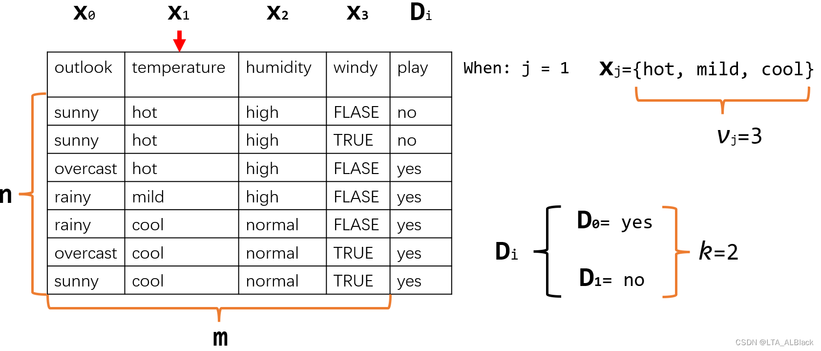
综上我们得到求解式5:\[d(\mathbf{x})=\underset{1 \leq i \leq k}{\arg \max } P\left(D_{i} \mid \mathbf{x}\right)=\underset{1 \leq i \leq k}{\arg \max } P\left(D_{i}\right) \prod_{j=1}^{m} P\left(x_{j} \mid D_{i}\right) \tag{5}\] \(d(\mathbf{x})\)表示的是当前最佳判决属性的下标,这个说起来很空,那我们的数据集举例子,我们的最佳判决属性是一个长度为2的数组Judge(即上式中\(k=2\)),Judge[0]为不去玩,Judge[1]为去玩,当返回的\(d(\mathbf{x}) = 1\)时就是去玩。显然,\(d(\mathbf{x})\)只能返回这两种情况。
· 基于程序设计的算法调整
算式5当中有大量概率相乘的情况,因为这里概率都是小于1的,所以最终的结果可能是一个非常小的数,对于计算机来说,这存在越界风险。于是我们可以通过log运算放大这个结果,同时因为log是单调递增的函数,对于多个要比大小的数据来说,这并不改变数据相互的大小关系,可以引用于\(\arg \max\)方法(这是数学公式到计算机中进行适应性的惯用伎俩!)\[d(\mathbf{x})=\underset{1 \leq i \leq k}{\arg \max } P\left(D_{i}\right) \prod_{j=1}^{m} P\left(x_{j} \mid D_{i}\right)=\underset{1 \leq i \leq k}{\arg \max }\left(\log P\left(D_{i}\right)+\sum_{j=1}^{m} \log P\left(x_{j} \mid D_{i}\right)\right) \tag{6}\] 注意log的基本运算法则(初中知识哦~)
· Laplacian 平滑
上面的log代替合理吗?log的定义域是\((0, +∞)\),而一般的概率范围是\([0,+∞)\)。发现危险了吗?
只要条件可能性足够庞大,我们的数据集往往是难以囊括所有的条件,因此总会存在某些条件的计算并不能反应真实情况。例如我们这里的14行数据集中就没有天气多云(outlook = overcast)与不打球(play = no)同时出现的情况,那么这样的话就有\(P(\text { outlook }=\text { overcast } \mid \text { play }=\text { no })=0\),即不打球时天气一定不是多云。因此完全可能出现0概率!
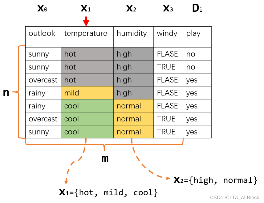
这样的数据显然是不对的,放到5式的累乘中,导致最终概率直接为0(一票否决现象),因此我们采用一种名为Laplacian平滑的方法\[P^{L}\left(x_{j} \mid D_{i}\right)=\frac{n P\left(x_{j} D_{i}\right)+1}{n P\left(D_{i}\right)+v_{j}} \tag{7}\] 这个式子是在原式:\( P\left(x_{j} \mid D_{i}\right)=\frac{P\left(x_{j} D_{i}\right)}{P\left(D_{i}\right)}\)的基础上改进得到的,目的在于极力避免0概率。这里\(v_j\)表示第\(j\)个\(x_j\)天气情况可能的分类,比如当前我们讨论的是XX决策下outlook天气情况,由\(outlook=\{sunny, overcast, rainy\}\),所以\(v_j = 3\)。
从效果上来看,\(v_j > 0\),而其余部分也没有出现负数的任何可能,定然\(P^{L}\left(x_{j} \mid D_{i}\right) > 0\),避免了0概率情况。
从理论上,是否能满足概率基本要求\(\sum^{v_j}_{j = 1}P^{L}\left(x_{j} \mid D_{i}\right) = 1\)呢?完全可以哟~ 分母的\(nP(D_i)\)其实就是全部数据行中\(D_i\)出现的行数,而\(nP(x_jD_i)\)表示全部数据行中那些同时满足\(x_j\)与\(D_i\)的数据行,如果遍历全部\(j\)可能的取值(假设数据列\(x_j\)有\(v_j\)种取值),相当于枚举了当前天气情况\(x_j\)的全部\(v_j\)种情况,自然\( \sum^{v_j}_{j = 1} nP(x_jD_i) = nP(D_i)\)。而分子中1枚举了\(v_j\)次,所以总的来说,分子通过累加后,与分母完全一致!
当然,除了\(P\left(x_{j} \mid D_{i}\right)\)要平滑,6式中的\(P(D_i)\)也需要平滑。\[P^{L}\left(D_{i}\right)=\frac{n P\left(D_{i}\right)+1}{n+k} \tag{8}\]
综上,我的得到算法需要实现的最终表达式\[d(\mathbf{x})=\underset{1 \leq i \leq k}{\arg \max } \log P^{L}\left(D_{i}\right)+\sum_{j=1}^{m} \log P^{L}\left(x_{j} \mid D_{i}\right) \tag{9}\]
二、代码的变量确定
    /**
	 * The number of classes. For binary classification it is 2.
	 */
	int numClasses;

	/**
	 * The number of instances.
	 */
	int numInstances;

	/**
	 * The number of conditional attributes.
	 */
int numConditions;- 第一个表示我们决策列具有的类别数目,就是我们公式中的\(k\)。本数据集中决策数据列足有yes与no俩情况,故\(k=2\)
- 第二个表示表的数据行个数,即公式中的\(n\)。
- 条件数目,即\(m\),是除开最后的决策列之后的常规训练的属性列。
    /**
	 * The prediction, including queried and predicted labels.
	 */
	int[] predicts;

	/**
	 * Class distribution.
	 */
	double[] classDistribution;

	/**
	 * Class distribution with Laplacian smooth.
	 */
double[] classDistributionLaplacian;- 第一个预测数组是一个长度为\(n\)预测数组,用于存放对于每一行数据进行leave-one-out测试时存放的预测结果。
- 第二个是\(P(D_i)\),因为我们数据集中\(k=2\),故这个数组长度也为2
- 第三个是\(P^{L}(D_i)\),因为我们数据集中\(k=2\),故这个数组长度也为2
	/**
	 * To calculate the conditional probabilities for all classes over all
	 * attributes on all values.
	 */
	double[][][] conditionalCounts;

	/**
	 * The conditional probabilities with Laplacian smooth.
	 */
	double[][][] conditionalProbabilitiesLaplacian;
这里的两个数据都是三维数组,他们都是通过三个维度来确定地定位到概率计算中的一些特性:
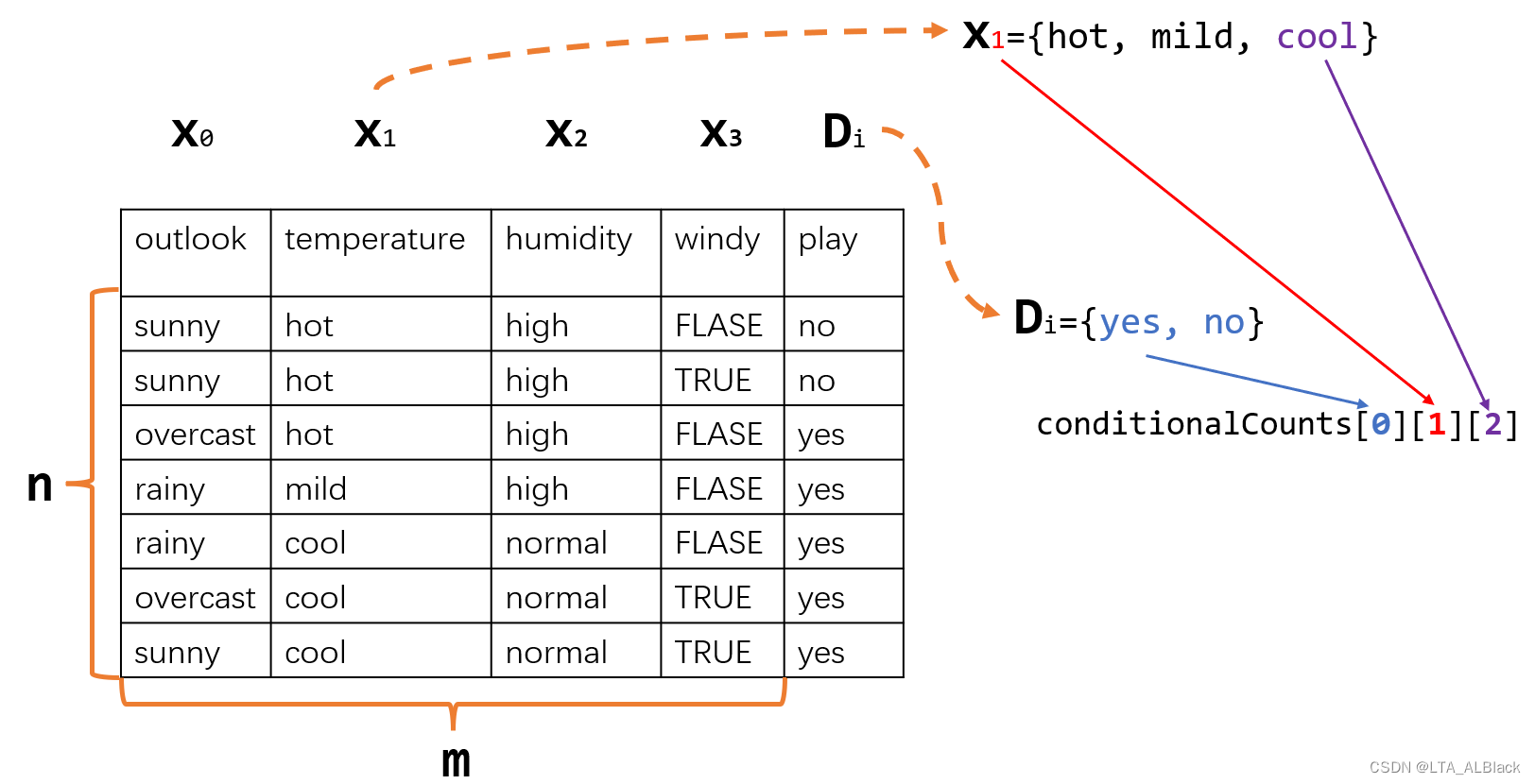
conditionCounts[0][1][2]++ 表示数据集又新找到了一个决策为出去玩,而且气温温度为凉爽的数据行,即conditionCounts[i][j][k]表示采用第i个决策并且当天的天气第j特征为第k种的数目。而conditionProbabilitiesLaplacian[i][j][]表示\(P^{L}(x_j |D_i)\),你可能疑问,第三维度呢?第三维度其实隐含在\(x_j\)里面,若实在难以理解,可以认为conditionProbabilitiesLaplacian[i][j][k]表示\(P^{L}((x_j = k) | D_i)\)的概率,比如conditionProbabilitiesLaplacian[0][1][2]就是,在某天出去玩的条件下,同时气温是凉爽的概率。
	/**
	 * Data type.
	 */
	int dataType;

	/**
	 * Nominal.
	 */
	public static final int NOMINAL = 0;

	/**
	 * Numerical.
	 */
	public static final int NUMERICAL = 1;
设置适用于什么类型的NB算法,0表示字符型,也就是今天的内容,1表示的数值型NB明天再看吧。
三、代码实现
1.构造函数
    /**
	 ********************
	 * The constructor.
	 *
	 * @param paraFilename
	 *            The given file.
	 ********************
	 */
	public NaiveBayes(String paraFilename) {
		dataset = null;
		try {
			FileReader fileReader = new FileReader(paraFilename);
			dataset = new Instances(fileReader);
			fileReader.close();
		} catch (Exception ee) {
			System.out.println("Cannot read the file: " + paraFilename + "\r\n" + ee);
			System.exit(0);
		} // Of try

		dataset.setClassIndex(dataset.numAttributes() - 1);
		numConditions = dataset.numAttributes() - 1;
		numInstances = dataset.numInstances();
		numClasses = dataset.attribute(numConditions).numValues();
	}// Of the constructor
构造函数主要完成数据的输入,确定决策类,然后逐次给类的数学\(n\)、\(m\)、\(k\)初始化。
2.计算\(P^{L}(D_i)\)
通过式8可以知道我们需要求什么,\(n\)与决策列的类别\(k\)都是已知的,只需要计算\(P(D_i)\),而这个概率计算只需要算\(D_i\)在数据行中出现的频度就好了。
/**
********************
* Calculate the class distribution with Laplacian smooth.
********************
*/
public void calculateClassDistribution() {
classDistribution = new double[numClasses];
classDistributionLaplacian = new double[numClasses];
double[] tempCounts = new double[numClasses];
for (int i = 0; i < numInstances; i++) {
int tempClassValue = (int) dataset.instance(i).classValue();
tempCounts[tempClassValue]++;
} // Of for i
for (int i = 0; i < numClasses; i++) {
classDistribution[i] = tempCounts[i] / numInstances;
classDistributionLaplacian[i] = (tempCounts[i] + 1) / (numInstances + numClasses);
} // Of for i
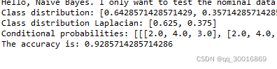
System.out.println("Class distribution: " + Arrays.toString(classDistribution));
System.out.println(
"Class distribution Laplacian: " + Arrays.toString(classDistributionLaplacian));
}// Of calculateClassDistribution这里初始化了一个长度为numClasses(公式中的\(k\))的桶tempCounts[],来统计对应的决策列属性出现的次数,也就是频度。循环中取出决策的所有类别,并计算有classDistribution[i] = tempCounts[i] / numInstances 这就是经典的古典概率的除法运算,以此得到\(P(D_i)\)。之后通过\(P(D_i)\)计算出\(P^{L}(D_i)\)。
可以发现这里\(P^{L}(D_i)\)的分支部分并没有乘\(n\),这其实避免了冗余,如果你完整第按照公式8来写就是:
classDistributionLaplacian[i] = (numInstances * classDistribution[i] + 1) / (numInstances + numClasses);而classDistribution[i]又可写作tempCounts[i] / numInstances,因此numInstances完全可以消掉。其实拉普拉斯平滑的目的本身就是将分子分母转化为确定条件的具体频度而避免0概率的,所以本质上它就是利用的符合的数据行数目而非概率。
3.计算\(P^{L}(x_j|D_i)\)
    /**
	 ********************
	 * Calculate the conditional probabilities with Laplacian smooth. ONLY scan
	 * the dataset once. There was a simpler one, I have removed it because the
	 * time complexity is higher.
	 ********************
	 */
	public void calculateConditionalProbabilities() {
		conditionalCounts = new double[numClasses][numConditions][];
		conditionalProbabilitiesLaplacian = new double[numClasses][numConditions][];

		// Allocate space
		for (int i = 0; i < numClasses; i++) {
			for (int j = 0; j < numConditions; j++) {
				int tempNumValues = (int) dataset.attribute(j).numValues();
				conditionalCounts[i][j] = new double[tempNumValues];
				conditionalProbabilitiesLaplacian[i][j] = new double[tempNumValues];
			} // Of for j
		} // Of for i

		// Count the numbers
		int[] tempClassCounts = new int[numClasses];
		for (int i = 0; i < numInstances; i++) {
			int tempClass = (int) dataset.instance(i).classValue();
			tempClassCounts[tempClass]++;
			for (int j = 0; j < numConditions; j++) {
				int tempValue = (int) dataset.instance(i).value(j);
				conditionalCounts[tempClass][j][tempValue]++;
			} // Of for j
		} // Of for i

		// Now for the real probability with Laplacian
		for (int i = 0; i < numClasses; i++) {
			for (int j = 0; j < numConditions; j++) {
				int tempNumValues = (int) dataset.attribute(j).numValues();
				for (int k = 0; k < tempNumValues; k++) {
					conditionalProbabilitiesLaplacian[i][j][k] = (conditionalCounts[i][j][k] + 1)
							/ (tempClassCounts[i] + tempNumValues);
				} // Of for k
			} // Of for j
		} // Of for i

		System.out.println("Conditional probabilities: " + Arrays.deepToString(conditionalCounts));
}// Of calculateConditionalProbabilities- 第7、8行的初始化并没有给出第三个维的初始化,这是因为第三维度是对应非决策列能表示的不同类别个数,这个是随不同列而不同的,因此无法确定的初始化。而第一维度——决策列的类别数目(代码中的numClasses,公式中的\(k\))是确定的,第二维度——非决策列个数(代码中numConditions,公式中\(m\))也是确定的。
- 第一个循环体,12~19行代码,就是逐步遍历每个可变的非决策条件列,然后确定其拥有的属性数目,并为其分配空间。
- 第二个循环体,21~30行代码,一行一行扫描数据集表格,顺便获知此行的决策情况(yes or no),同时顺便统计不同决策的频度于tempClassCount。当然,最主要的任务还是依次取出这一个行的每个非决策条件列,计数于三位数组conditionCounts。
- 第三个循环体,32~41行代码,逐行扫描,并且分析逐行每个决策情况、条件情况,并且计算\(P^{L}(x_j|D_i)\)。
4.计算\(d(\mathbf{x})\)
参考上文的公式9:\[d(\mathbf{x})=\underset{1 \leq i \leq k}{\arg \max } \log P^{L}\left(D_{i}\right)+\sum_{j=1}^{m} \log P^{L}\left(x_{j} \mid D_{i}\right) \] \(P^{L}\left(x_{j}|D_{i}\right)\)已经存储于三维数组之中conditionalProbabilitiesLaplacian。而 \(P^{L}\left(D_{i}\right)\)也已经存储好,因此,直接带入计算即可:
	/**
	 ********************
	 * Classify an instances with nominal data.
	 ********************
	 */
	public int classifyNominal(Instance paraInstance) {
		// Find the biggest one
		double tempBiggest = -10000;
		int resultBestIndex = 0;
		for (int i = 0; i < numClasses; i++) {
			double tempClassProbabilityLaplacian = Math.log(classDistributionLaplacian[i]);
			double tempPseudoProbability = tempClassProbabilityLaplacian;
			for (int j = 0; j < numConditions; j++) {
				int tempAttributeValue = (int) paraInstance.value(j);

				// Laplacian smooth.
				tempPseudoProbability += Math.log(conditionalProbabilitiesLaplacian[i][j][tempAttributeValue]);
			} // Of for j

			if (tempBiggest < tempPseudoProbability) {
				tempBiggest = tempPseudoProbability;
				resultBestIndex = i;
			} // Of if
		} // Of for i

		return resultBestIndex;
	}// Of classifyNominal
5.其余函数以及运行框架
其余框架相比来说重要性已经不高了,贴出来即可。最终我们是将leave-one-out测试后的预测数据存放于predicts数组之中,最后算精度的时候类似于KNN,计算正确的个数占总数的比重。
	/**
	 ********************
	 * Classify all instances, the results are stored in predicts[].
	 ********************
	 */
	public void classify() {
		predicts = new int[numInstances];
		for (int i = 0; i < numInstances; i++) {
			predicts[i] = classify(dataset.instance(i));
		} // Of for i
	}// Of classify

	/**
	 ********************
	 * Classify an instances.
	 ********************
	 */
	public int classify(Instance paraInstance) {
		if (dataType == NOMINAL) {
			return classifyNominal(paraInstance);
		} else if (dataType == NUMERICAL) {
			return classifyNumerical(paraInstance);
		} // Of if

		return -1;
	}// Of classify
	/**
	 ********************
	 * Compute accuracy.
	 ********************
	 */
	public double computeAccuracy() {
		double tempCorrect = 0;
		for (int i = 0; i < numInstances; i++) {
			if (predicts[i] == (int) dataset.instance(i).classValue()) {
				tempCorrect++;
			} // Of if
		} // Of for i

		double resultAccuracy = tempCorrect / numInstances;
		return resultAccuracy;
	}// Of computeAccuracy
    /**
	 *************************
	 * Test nominal data.
	 *************************
	 */
	public static void testNominal() {
		System.out.println("Hello, Naive Bayes. I only want to test the nominal data.");
		String tempFilename = "D:/Java DataSet/weather.arff";

		NaiveBayes tempLearner = new NaiveBayes(tempFilename);
		tempLearner.setDataType(NOMINAL);
		tempLearner.calculateClassDistribution();
		tempLearner.calculateConditionalProbabilities();
		tempLearner.classify();

		System.out.println("The accuracy is: " + tempLearner.computeAccuracy());
	}// Of testNominal
    /**
	 *************************
	 * Test this class.
	 *
	 * @param args
	 *            Not used now.
	 *************************
	 */
	public static void main(String[] args) {
		testNominal();
	}// Of main
四、运行测试
天气数据的效果还不错呢,但是这个数据量还是太小了,为了更进一步,我试了下老师的mushroom.arff数据(这个数据集大概有8000多数据,下载:https://gitee.com/fansmale/javasampledata)
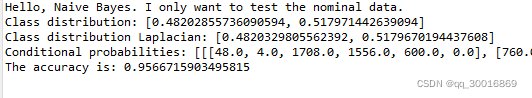
可以发现,数据的准确度接近1.0,NB算法效果还是非常不错的。明天试着完成数值型数据的NB算法,从而和我们之前讲的KNN分类算法进行一下同行之间的比对。