动手学深度学习第五章

5.1

def corr2d(X, K):
    h, w = K.shape
    Y = tf.Variable(tf.zeros((X.shape[0] - h + 1, X.shape[1] - w +1)))
    for i in range(Y.shape[0]):
        for j in range(Y.shape[1]):
            Y[i,j].assign(tf.cast(tf.reduce_sum(X[i:i+h, j:j+w] * K), dtype=tf.float32))
    return Y
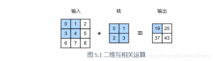
X = tf.constant([[0,1,2], [3,4,5], [6,7,8]])
K = tf.constant([[0,1], [2,3]])
corr2d(X, K)

这个代码是卷积的实现

<tf.Variable 'Variable:0' shape=(2, 2) dtype=float32, numpy=
array([[19., 25.],
       [37., 43.]], dtype=float32)>

class Conv2D(tf.keras.layers.Layer):
    def __init__(self, units):
        super().__init__()
        self.units = units

    def build(self, kernel_size):
        self.w = self.add_weight(name='w',
                                shape=kernel_size,
                                initializer=tf.random_normal_initializer())
        self.b = self.add_weight(name='b',
                                shape=(1,),
                                initializer=tf.random_normal_initializer())
    def call(self, inputs):
        return corr2d(inputs, self.w) + self.b

init()：保存成员变量的设置
build()：在call()函数第一次执行时会被调用一次，这时候可以知道输入数据的shape。返回去看一看，果然是__init__()函数中只初始化了输出数据的shape，而输入数据的shape需要在build()函数中动态获取，这也解释了为什么在有__init__()函数时还需要使用build()函数
call()： call()函数就很简单了，即当其被调用时会被执行。
https://www.cnblogs.com/yinyoupoet/p/13287358.html

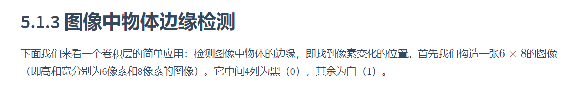
X = tf.Variable(tf.ones((6,8)))#创建一个变量
X[:, 2:6].assign(tf.zeros(X[:,2:6].shape))#对变量进行赋值
X

<tf.Variable 'Variable:0' shape=(6, 8) dtype=float32, numpy=
array([[1., 1., 0., 0., 0., 0., 1., 1.],
       [1., 1., 0., 0., 0., 0., 1., 1.],
       [1., 1., 0., 0., 0., 0., 1., 1.],
       [1., 1., 0., 0., 0., 0., 1., 1.],
       [1., 1., 0., 0., 0., 0., 1., 1.],
       [1., 1., 0., 0., 0., 0., 1., 1.]], dtype=float32)>

然后我们构造一个高和宽分别为1和2的卷积核K。当它与输入做互相关运算时，如果横向相邻元素相同，输出为0；否则输出为非0。

K = tf.constant([[1,-1]], dtype = tf.float32)

下面将输入X和我们设计的卷积核K做互相关运算。可以看出，我们将从白到黑的边缘和从黑到白的边缘分别检测成了1和-1。其余部分的输出全是0。

Y = corr2d(X, K)
Y

<tf.Variable 'Variable:0' shape=(6, 7) dtype=float32, numpy=
array([[ 0.,  1.,  0.,  0.,  0., -1.,  0.],
       [ 0.,  1.,  0.,  0.,  0., -1.,  0.],
       [ 0.,  1.,  0.,  0.,  0., -1.,  0.],
       [ 0.,  1.,  0.,  0.,  0., -1.,  0.],
       [ 0.,  1.,  0.,  0.,  0., -1.,  0.],
       [ 0.,  1.,  0.,  0.,  0., -1.,  0.]], dtype=float32)>

使用tf.keras.layers提供的Conv2D类来实现卷积核更新。

# 二维卷积层使用4维输入输出，格式为(样本, 高, 宽, 通道)，这里批量大小（批量中的样本数）和通道数均为1
X = tf.reshape(X, (1,6,8,1))
Y = tf.reshape(Y, (1,6,7,1))
Y

# 构造一个输出通道数为1（将在“多输入通道和多输出通道”一节介绍通道），核数组形状是(1, 2)的二维卷积层
conv2d = tf.keras.layers.Conv2D(1, (1,2))
#input_shape = (samples, rows, cols, channels)
# Y = conv2d(X)
Y.shape

Y_hat = conv2d(X)
for i in range(10):
    with tf.GradientTape(watch_accessed_variables=False) as g:
        g.watch(conv2d.weights[0])
        Y_hat = conv2d(X)
        l = (abs(Y_hat - Y)) ** 2
        dl = g.gradient(l, conv2d.weights[0])
        lr = 3e-2
        update = tf.multiply(lr, dl)
        updated_weights = conv2d.get_weights()
        updated_weights[0] = conv2d.weights[0] - update
        conv2d.set_weights(updated_weights)  

        if (i + 1)% 2 == 0:
            print('batch %d, loss %.3f' % (i + 1, tf.reduce_sum(l)))

Y_hat = conv2d(X)
for i in range(10):
    with tf.GradientTape(watch_accessed_variables=False) as g:
        g.watch(conv2d.weights[0])
        Y_hat = conv2d(X)
        l = (abs(Y_hat - Y)) ** 2
        dl = g.gradient(l, conv2d.weights[0])
        lr = 3e-2
        update = tf.multiply(lr, dl)
        updated_weights = conv2d.get_weights()
        updated_weights[0] = conv2d.weights[0] - update
        conv2d.set_weights(updated_weights)  

        if (i + 1)% 2 == 0:
            print('batch %d, loss %.3f' % (i + 1, tf.reduce_sum(l)))

batch 2, loss 0.235
batch 4, loss 0.041
batch 6, loss 0.008
batch 8, loss 0.002
batch 10, loss 0.000

可以看到，10次迭代后误差已经降到了一个比较小的值。现在来看一下学习到的核数组。

tf.reshape(conv2d.get_weights()[0],(1,2))

<tf.Tensor: id=1012, shape=(1, 2), dtype=float32, numpy=array([[ 0.99903595, -0.9960023 ]], dtype=float32)>

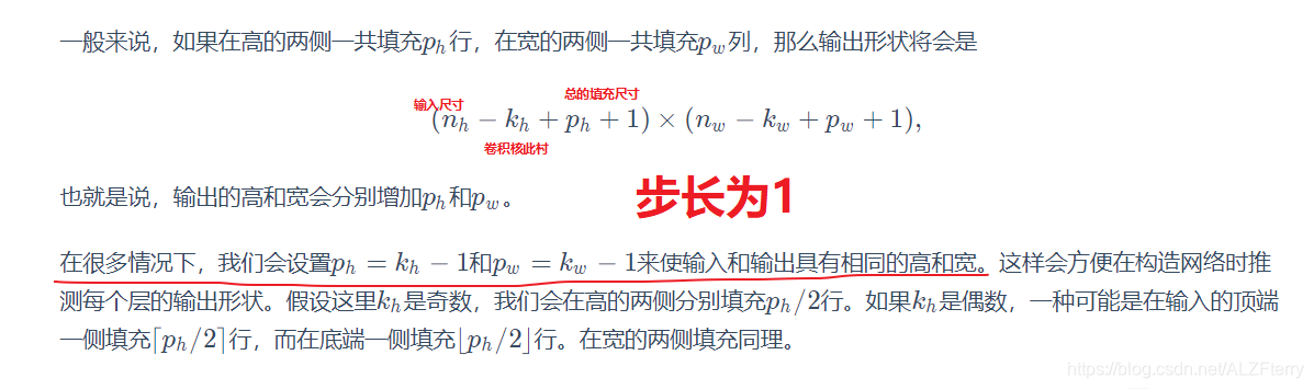
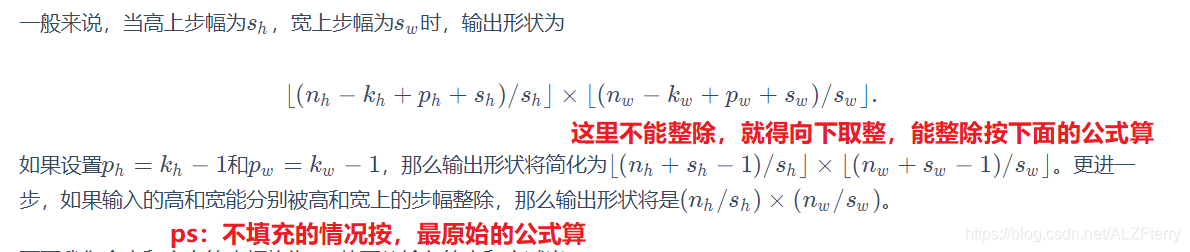
5.2 填充和步幅

https://blog.csdn.net/ALZFterry/article/details/109105829
这章节，主要讲解填充后，和步幅为2后，输出特征图尺寸的大小。

def comp_conv2d(conv2d, X):
    X = tf.reshape(X,(1,) + X.shape + (1,))#
    #这句话，在最前，最后增加了维度，第一次见这么使用的，增加后的维度为（1，8，8，1）
    Y = conv2d(X)
    #input_shape = (samples, rows, cols, channels)
    return tf.reshape(Y,Y.shape[1:3])

conv2d = tf.keras.layers.Conv2D(1, kernel_size=3, padding='same')
X = tf.random.uniform(shape=(8,8))
comp_conv2d(conv2d,X).shape

TensorShape([8, 8])

5.3

def corr2d(X, K):
    h, w = K.shape
    if len(X.shape) <= 1:
        X = tf.reshape(X, (X.shape[0],1))
    Y = tf.Variable(tf.zeros((X.shape[0] - h + 1, X.shape[1] - w +1)))
    for i in range(Y.shape[0]):
        for j in range(Y.shape[1]):
            Y[i,j].assign(tf.cast(tf.reduce_sum(X[i:i+h, j:j+w] * K), dtype=tf.float32))
    return Y

实现：

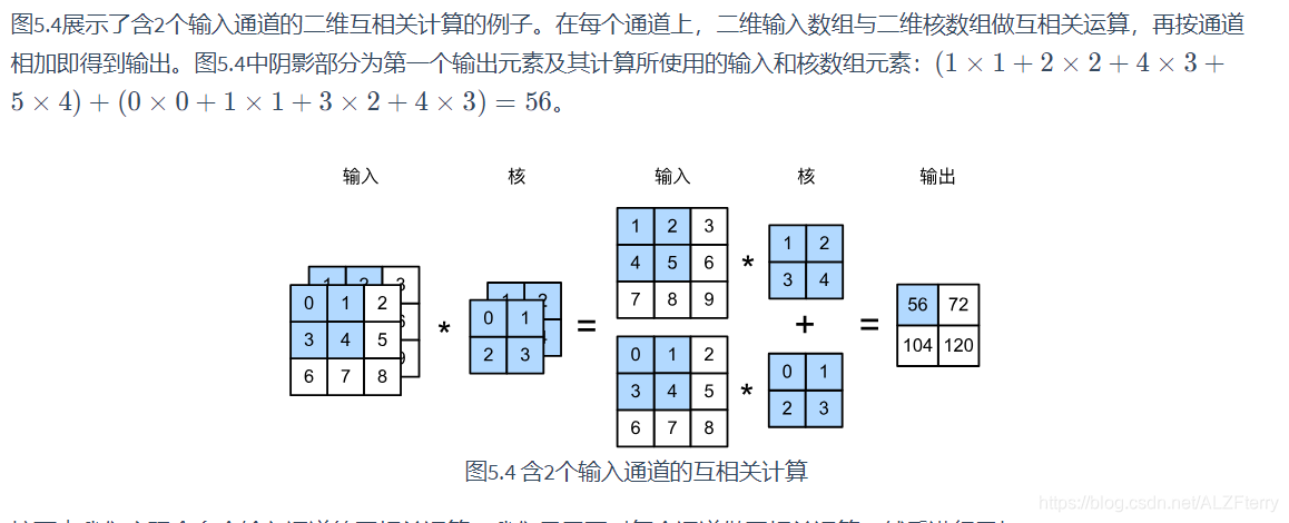
def corr2d_multi_in(X, K):
    return tf.reduce_sum([corr2d(X[i], K[i]) for i in range(X.shape[0])],axis=0)

X = tf.constant([[[0,1,2],[3,4,5],[6,7,8]],
                 [[1,2,3],[4,5,6],[7,8,9]]])
K = tf.constant([[[0,1],[2,3]],
                 [[1,2],[3,4]]])

corr2d_multi_in(X, K)

<tf.Tensor: id=145, shape=(2, 2), dtype=float32, numpy=
array([[ 56.,  72.],
       [104., 120.]], dtype=float32)>

上面输出的的大小通道数均为1，要想通道数增加，那么需要增加卷积核的个数。

def corr2d_multi_in_out(X, K):
    # 对K的第0维遍历，每次同输入X做互相关计算。所有结果使用stack函数合并在一起
    return tf.stack([corr2d_multi_in(X, k) for k in K],axis=0)

K = tf.stack([K, K+1, K+2],axis=0)
K.shape

TensorShape([3, 2, 2, 2])

corr2d_multi_in_out(X, K)

<tf.Tensor: id=592, shape=(3, 2, 2), dtype=float32, numpy=
array([[[ 56.,  72.],
        [104., 120.]],

       [[ 76., 100.],
        [148., 172.]],

       [[ 96., 128.],
        [192., 224.]]], dtype=float32)>

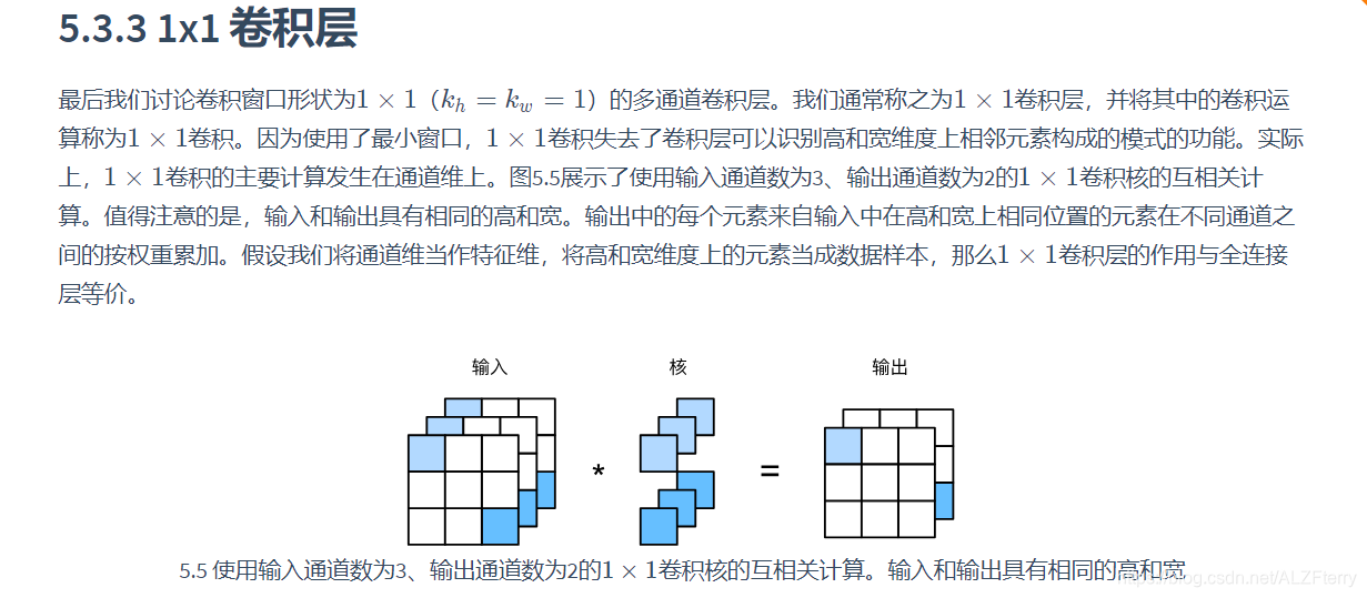
实现：

def corr2d_multi_in_out_1x1(X, K):
    c_i, h, w = X.shape
    c_o = K.shape[0]
    X = tf.reshape(X,(c_i, h * w))
    K = tf.reshape(K,(c_o, c_i))
    Y = tf.matmul(K, X)
    return tf.reshape(Y, (c_o, h, w))

X = tf.random.uniform((3,3,3))
K = tf.random.uniform((2,3,1,1))

Y1 = corr2d_multi_in_out_1x1(X, K)
Y2 = corr2d_multi_in_out(X, K)

tf.norm(Y1-Y2) < 1e-6

<tf.Tensor: id=1392, shape=(), dtype=bool, numpy=True>

5.4

池化（pooling）层，它的提出是为了缓解卷积层对位置的过度敏感性。

def pool2d(X, pool_size, mode='max'):
    p_h, p_w = pool_size
    Y = tf.zeros((X.shape[0] - p_h + 1, X.shape[1] - p_w +1))
    Y = tf.Variable(Y)
    for i in range(Y.shape[0]):
        for j in range(Y.shape[1]):
            if mode == 'max':
                Y[i,j].assign(tf.reduce_max(X[i:i+p_h, j:j+p_w]))
            elif mode =='avg':
                Y[i,j].assign(tf.reduce_mean(X[i:i+p_h, j:j+p_w]))
    return Y

我们可以构造图5.6中的输入数组X来验证二维最大池化层的输出。

X = tf.constant([[0,1,2],[3,4,5],[6,7,8]],dtype=tf.float32)
pool2d(X, (2,2))

<tf.Variable 'Variable:0' shape=(2, 2) dtype=float32, numpy=
array([[4., 5.],
       [7., 8.]], dtype=float32)>

同时我们实验一下平均池化层。

pool2d(X, (2,2), 'avg')

<tf.Variable 'Variable:0' shape=(2, 2) dtype=float32, numpy=
array([[2., 3.],
       [5., 6.]], dtype=float32)>

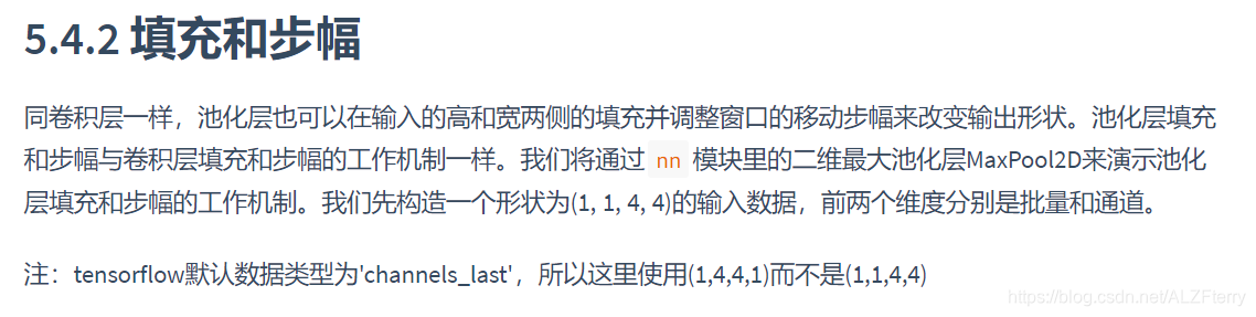
#tensorflow default data_format == 'channels_last'
#so (1,4,4,1) instead of (1,1,4,4)
X = tf.reshape(tf.constant(range(16)), (1,4,4,1))
X

<tf.Tensor: id=112, shape=(1, 4, 4, 1), dtype=int32, numpy=
array([[[[ 0],
         [ 1],
         [ 2],
         [ 3]],

        [[ 4],
         [ 5],
         [ 6],
         [ 7]],

        [[ 8],
         [ 9],
         [10],
         [11]],

        [[12],
         [13],
         [14],
         [15]]]])>

默认情况下，MaxPool2D实例里步幅和池化窗口形状相同。下面使用形状为(3, 3)的池化窗口，默认获得形状为(3, 3)的步幅。

pool2d = tf.keras.layers.MaxPool2D(pool_size=[3,3])
pool2d(X)

<tf.Tensor: id=113, shape=(1, 1, 1, 1), dtype=int32, numpy=array([[[[10]]]])>

上面这个不知道为什么是这样

# tensorflow 中 padding 有 same 和 valid 两种， same 会在窗口大小不满足时填充0，valid 会舍弃即不填充
# one of "valid" or "same" (case-insensitive). "valid" means no padding. "same" results in padding evenly to the left/right or up/down of the input such that output has the same height/width dimension as the input

pool2d = tf.keras.layers.MaxPool2D(pool_size=[3,3],padding='same',strides=2)
pool2d(X)

<tf.Tensor: id=114, shape=(1, 2, 2, 1), dtype=int32, numpy=
array([[[[10],
         [11]],

        [[14],
         [15]]]])>

上面这个不知道为什么是这样

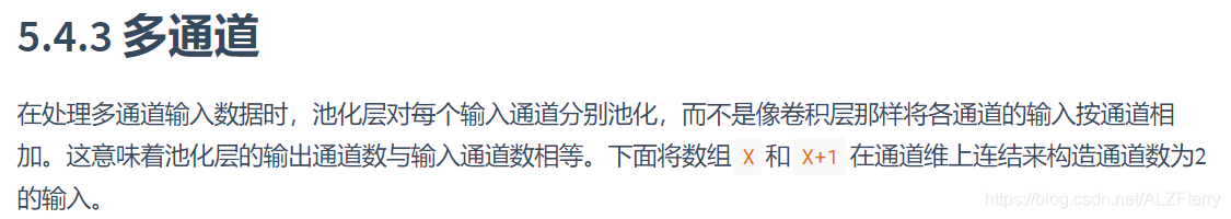
X = tf.concat([X, X+1], axis=3)
X.shape

TensorShape([1, 4, 4, 2])

池化后，我们发现输出通道数仍然是2。

pool2d = tf.keras.layers.MaxPool2D(3, padding='same', strides=2)
pool2d(X)

<tf.Tensor: shape=(1, 2, 2, 2), dtype=int32, numpy=
array([[[[10, 11],
         [11, 12]],

        [[14, 15],
         [15, 16]]]])>

5.5 LeNet

LeNet分为卷积层块和全连接层块两个部分。下面我们分别介绍这两个模块。

卷积层块里的基本单位是卷积层后接最大池化层：卷积层用来识别图像里的空间模式，如线条和物体局部，之后的最大池化层则用来降低卷积层对位置的敏感性。卷积层块由两个这样的基本单位重复堆叠构成。在卷积层块中，每个卷积层都使用55的窗口，并在输出上使用sigmoid激活函数。第一个卷积层输出通道数为6，第二个卷积层输出通道数则增加到16。这是因为第二个卷积层比第一个卷积层的输入的高和宽要小，所以增加输出通道使两个卷积层的参数尺寸类似。卷积层块的两个最大池化层的窗口形状均为22，且步幅为2。由于池化窗口与步幅形状相同，池化窗口在输入上每次滑动所覆盖的区域互不重叠。

卷积层块的输出形状为(批量大小, 通道, 高, 宽)。当卷积层块的输出传入全连接层块时，全连接层块会将小批量中每个样本变平（flatten）。也就是说，全连接层的输入形状将变成二维，其中第一维是小批量中的样本，第二维是每个样本变平后的向量表示，且向量长度为通道、高和宽的乘积。全连接层块含3个全连接层。它们的输出个数分别是120、84和10，其中10为输出的类别个数。

import tensorflow as tf
import numpy as np


net = tf.keras.models.Sequential([
    tf.keras.layers.Conv2D(filters=6,kernel_size=5,activation='sigmoid',input_shape=(28,28,1)),
    tf.keras.layers.MaxPool2D(pool_size=2, strides=2),
    tf.keras.layers.Conv2D(filters=16,kernel_size=5,activation='sigmoid'),
    tf.keras.layers.MaxPool2D(pool_size=2, strides=2),
    tf.keras.layers.Flatten(),
    tf.keras.layers.Dense(120,activation='sigmoid'),
    tf.keras.layers.Dense(84,activation='sigmoid'),
    tf.keras.layers.Dense(10,activation='sigmoid')
])
X = tf.random.uniform((1,28,28,1))
for layer in net.layers:
    X = layer(X)
    print(layer.name, 'output shape\t', X.shape)
fashion_mnist = tf.keras.datasets.fashion_mnist

(train_images, train_labels), (test_images, test_labels) = fashion_mnist.load_data()
train_images = tf.reshape(train_images, (train_images.shape[0],train_images.shape[1],train_images.shape[2], 1))
print(train_images.shape)

test_images = tf.reshape(test_images, (test_images.shape[0],test_images.shape[1],test_images.shape[2], 1))
optimizer = tf.keras.optimizers.SGD(learning_rate=0.9, momentum=0.0, nesterov=False)

net.compile(optimizer=optimizer,
              loss='sparse_categorical_crossentropy',
              metrics=['accuracy'])


net.fit(train_images, train_labels, epochs=5, validation_split=0.1)

net.summary() 这句话 可以把模型的参数大小打印出来。


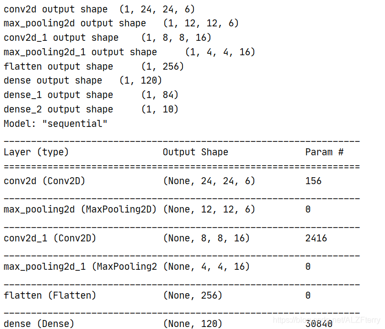
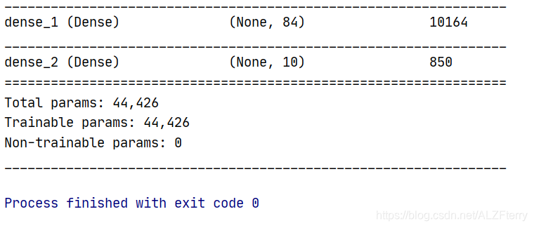
这里注意 参数的多少是怎么算出来的。

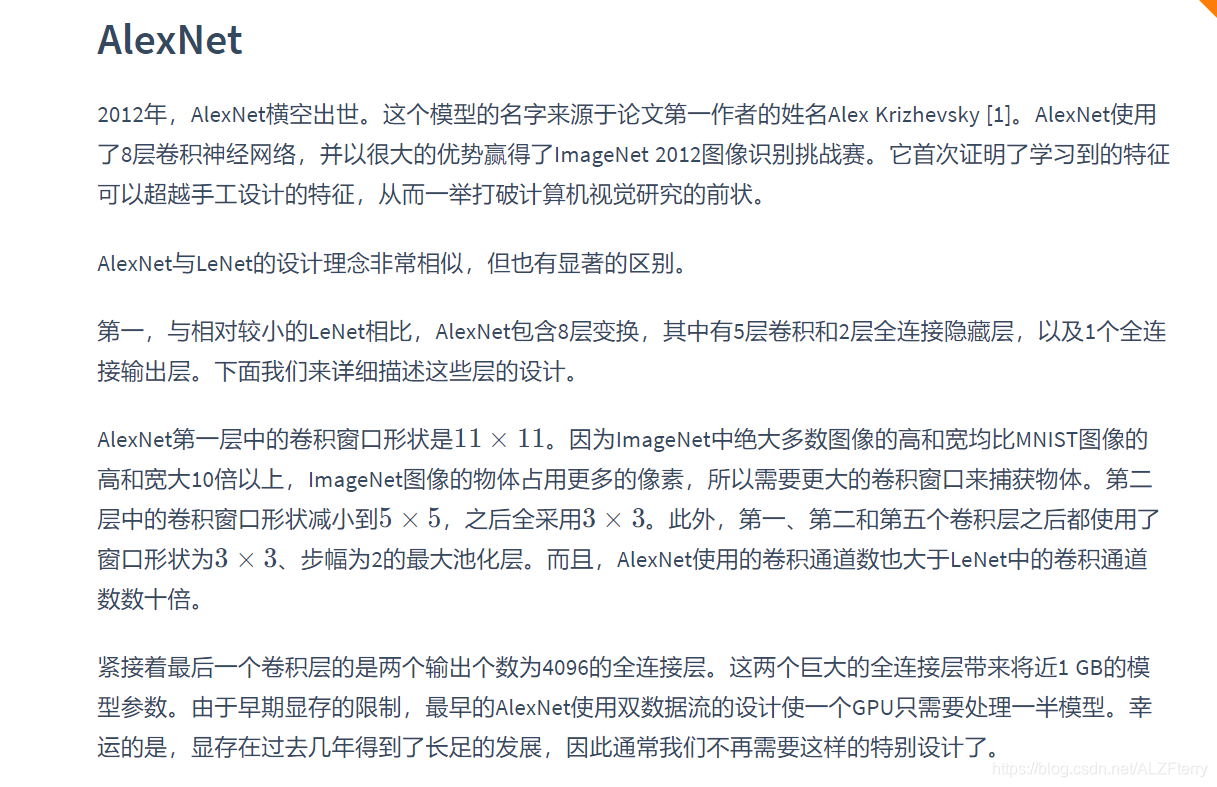
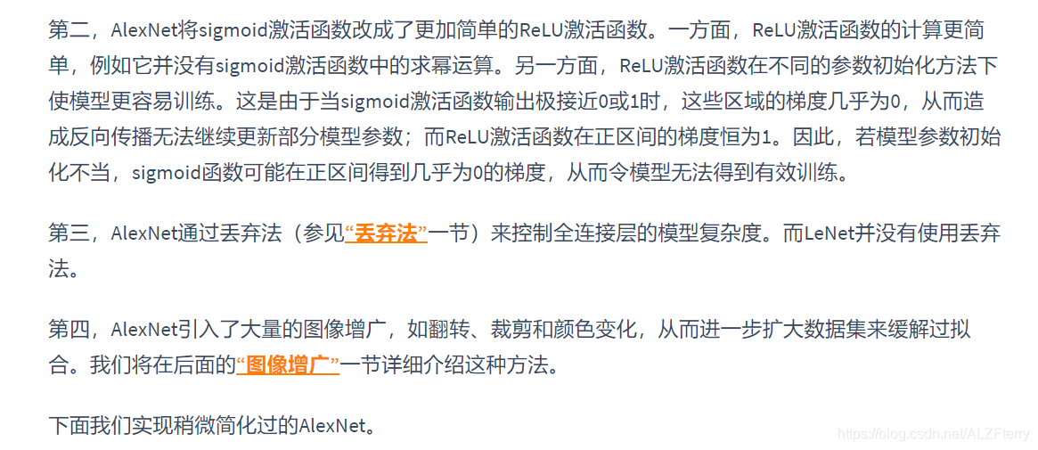
5.6 AlexNet

摘录 ：
特征如何表示：
在多层神经网络中，图像的第一级的表示可以是在特定的位置和⻆度是否出现边缘；而第二级的表示说不定能够将这些边缘组合出有趣的模式，如花纹；在第三级的表示中，也许上一级的花纹能进一步汇合成对应物体特定部位的模式。这样逐级表示下去，最终，模型能够较容易根据最后一级的表示完成分类任务。需要强调的是，输入的逐级表示由多层模型中的参数决定，而这些参数都是学出来的。

import tensorflow as tf
import numpy as np


net = tf.keras.models.Sequential([
    tf.keras.layers.Conv2D(filters=96,kernel_size=11,strides=4,activation='relu'),
    tf.keras.layers.MaxPool2D(pool_size=3, strides=2),
    tf.keras.layers.Conv2D(filters=256,kernel_size=5,padding='same',activation='relu'),
    tf.keras.layers.MaxPool2D(pool_size=3, strides=2),
    tf.keras.layers.Conv2D(filters=384,kernel_size=3,padding='same',activation='relu'),
    tf.keras.layers.Conv2D(filters=384,kernel_size=3,padding='same',activation='relu'),
    tf.keras.layers.Conv2D(filters=256,kernel_size=3,padding='same',activation='relu'),
    tf.keras.layers.MaxPool2D(pool_size=3, strides=2),
    tf.keras.layers.Flatten(),
    tf.keras.layers.Dense(4096,activation='relu'),
    tf.keras.layers.Dropout(0.5),
    tf.keras.layers.Dense(4096,activation='relu'),
    tf.keras.layers.Dropout(0.5),
    tf.keras.layers.Dense(10,activation='sigmoid')
])
X = tf.random.uniform((1,224,224,1))
for layer in net.layers:
    X = layer(X)
    print(layer.name, 'output shape\t', X.shape)
import numpy as np

class DataLoader():
    def __init__(self):
        fashion_mnist = tf.keras.datasets.fashion_mnist
        (self.train_images, self.train_labels), (self.test_images, self.test_labels) = fashion_mnist.load_data()
        self.train_images = np.expand_dims(self.train_images.astype(np.float32)/255.0,axis=-1)
        self.test_images = np.expand_dims(self.test_images.astype(np.float32)/255.0,axis=-1)
        self.train_labels = self.train_labels.astype(np.int32)
        self.test_labels = self.test_labels.astype(np.int32)
        self.num_train, self.num_test = self.train_images.shape[0], self.test_images.shape[0]

    def get_batch_train(self, batch_size):
        index = np.random.randint(0, np.shape(self.train_images)[0], batch_size)
        #need to resize images to (224,224)
        resized_images = tf.image.resize_with_pad(self.train_images[index],224,224,)
        return resized_images.numpy(), self.train_labels[index]

    def get_batch_test(self, batch_size):
        index = np.random.randint(0, np.shape(self.test_images)[0], batch_size)
        #need to resize images to (224,224)
        resized_images = tf.image.resize_with_pad(self.test_images[index],224,224,)
        return resized_images.numpy(), self.test_labels[index]

batch_size = 128
dataLoader = DataLoader()
x_batch, y_batch = dataLoader.get_batch_train(batch_size)
print("x_batch shape:",x_batch.shape,"y_batch shape:", y_batch.shape)



def train_alexnet():
    epoch = 5
    num_iter = dataLoader.num_train//batch_size
    for e in range(epoch):
        for n in range(num_iter):
            x_batch, y_batch = dataLoader.get_batch_train(batch_size)
            net.fit(x_batch, y_batch)
            if n%20 == 0:
                net.save_weights("5.6_alexnet_weights.h5")

optimizer = tf.keras.optimizers.SGD(learning_rate=0.01, momentum=0.0, nesterov=False)

net.compile(optimizer=optimizer,
              loss='sparse_categorical_crossentropy',
              metrics=['accuracy'])

x_batch, y_batch = dataLoader.get_batch_train(batch_size)
net.fit(x_batch, y_batch)
train_alexnet()

测试：

net.load_weights("5.6_alexnet_weights.h5")

x_test, y_test = dataLoader.get_batch_test(2000)
net.evaluate(x_test, y_test, verbose=2)

5.7VGG

import tensorflow as tf
print(tf.__version__)

for gpu in tf.config.experimental.list_physical_devices('GPU'):
    tf.config.experimental.set_memory_growth(gpu, True)

调用了 GPU

def vgg_block(num_convs, num_channels):
    blk = tf.keras.models.Sequential()
    for _ in range(num_convs):
        blk.add(tf.keras.layers.Conv2D(num_channels,kernel_size=3,
                                    padding='same',activation='relu'))

    blk.add(tf.keras.layers.MaxPool2D(pool_size=2, strides=2))
    return blk

下面我们实现VGG-11。

def vgg(conv_arch):
    net = tf.keras.models.Sequential()
    for (num_convs, num_channels) in conv_arch:
        net.add(vgg_block(num_convs,num_channels))
    net.add(tf.keras.models.Sequential([tf.keras.layers.Flatten(),
             tf.keras.layers.Dense(4096,activation='relu'),
             tf.keras.layers.Dropout(0.5),
             tf.keras.layers.Dense(4096,activation='relu'),
             tf.keras.layers.Dropout(0.5),
             tf.keras.layers.Dense(10,activation='sigmoid')]))
    return net

net = vgg(conv_arch)
X = tf.random.uniform((1,224,224,1))
for blk in net.layers:
    X = blk(X)
    print(blk.name, 'output shape:\t', X.shape)
    
ratio = 4
small_conv_arch = [(pair[0], pair[1] // ratio) for pair in conv_arch]
net = vgg(small_conv_arch)

数据加载

import numpy as np

class DataLoader():
    def __init__(self):
        fashion_mnist = tf.keras.datasets.fashion_mnist
        (self.train_images, self.train_labels), (self.test_images, self.test_labels) = fashion_mnist.load_data()
        self.train_images = np.expand_dims(self.train_images.astype(np.float32)/255.0,axis=-1)
        self.test_images = np.expand_dims(self.test_images.astype(np.float32)/255.0,axis=-1)
        self.train_labels = self.train_labels.astype(np.int32)
        self.test_labels = self.test_labels.astype(np.int32)
        self.num_train, self.num_test = self.train_images.shape[0], self.test_images.shape[0]

    def get_batch_train(self, batch_size):
        index = np.random.randint(0, np.shape(self.train_images)[0], batch_size)
        #need to resize images to (224,224)
        resized_images = tf.image.resize_with_pad(self.train_images[index],224,224,)
        return resized_images.numpy(), self.train_labels[index]

    def get_batch_test(self, batch_size):
        index = np.random.randint(0, np.shape(self.test_images)[0], batch_size)
        #need to resize images to (224,224)
        resized_images = tf.image.resize_with_pad(self.test_images[index],224,224,)
        return resized_images.numpy(), self.test_labels[index]

batch_size = 128
dataLoader = DataLoader()
x_batch, y_batch = dataLoader.get_batch_train(batch_size)
print("x_batch shape:",x_batch.shape,"y_batch shape:", y_batch.shape)

训练

def train_vgg():
#     net.load_weights("5.7_vgg_weights.h5")
    epoch = 5
    num_iter = dataLoader.num_train//batch_size
    for e in range(epoch):
        for n in range(num_iter):
            x_batch, y_batch = dataLoader.get_batch_train(batch_size)
            net.fit(x_batch, y_batch)
            if n%20 == 0:
                net.save_weights("5.7_vgg_weights.h5")

optimizer = tf.keras.optimizers.SGD(learning_rate=0.05, momentum=0.0, nesterov=False)

net.compile(optimizer=optimizer,
              loss='sparse_categorical_crossentropy',
              metrics=['accuracy'])

x_batch, y_batch = dataLoader.get_batch_train(batch_size)
net.fit(x_batch, y_batch)
train_vgg()

测试

net.load_weights("5.7_vgg_weights.h5")

x_test, y_test = dataLoader.get_batch_test(2000)
net.evaluate(x_test, y_test, verbose=2)

5.8NIN

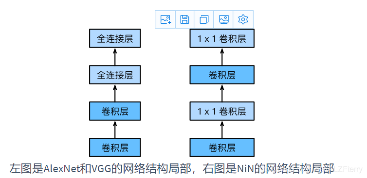
LeNet、AlexNet和VGG在设计上的共同之处是：先以由卷积层构成的模块充分抽取空间特征，再以由全连接层构成的模块来输出分类结果。其中，AlexNet和VGG对LeNet的改进主要在于如何对这两个模块加宽（增加通道数）和加深。本节我们介绍网络中的网络（NiN）[1]。它提出了另外一个思路，即串联多个由卷积层和“全连接”层构成的小网络来构建一个深层网络。

我们知道，卷积层的输入和输出通常是四维数组（样本，通道，高，宽），而全连接层的输入和输出则通常是二维数组（样本，特征）。如果想在全连接层后再接上卷积层，则需要将全连接层的输出变换为四维。
1×1卷积层。它可以看成全连接层，其中空间维度（高和宽）上的每个元素相当于样本，通道相当于特征。因此，NiN使用1×1卷积层来替代全连接层，从而使空间信息能够自然传递到后面的层中去。

代码略

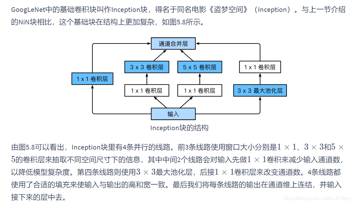
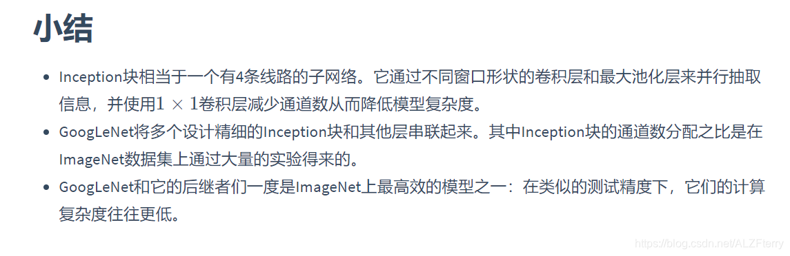
5.9GoogleNet

代码略

5.10 批归一化（BN）

通常来说，数据标准化预处理对于浅层模型就足够有效了。随着模型训练的进行，当每层中参数更新时，靠近输出层的输出较难出现剧烈变化。但对深层神经网络来说，即使输入数据已做标准化，训练中模型参数的更新依然很容易造成靠近输出层输出的剧烈变化。这种计算数值的不稳定性通常令我们难以训练出有效的深度模型。

批量归一化的提出正是为了应对深度模型训练的挑战。在模型训练时，批量归一化利用小批量上的均值和标准差，不断调整神经网络中间输出，从而使整个神经网络在各层的中间输出的数值更稳定。批量归一化和下一节将要介绍的残差网络为训练和设计深度模型提供了两类重要思路。
对全连接层做批量归一化：
我们先考虑如何对全连接层做批量归一化。通常，我们将批量归一化层置于全连接层中的仿射变换和激活函数之间。设全连接层的输入为$\mathbf{u}$，权重参数和偏差参数分别为$\mathbf{W}$和$\mathbf{b}$，，激活函数为ϕ。设批量归一化的运算符为$\mathbf{B}\mathbf{N}$。那么，使用批量归一化的全连接层的输出为：
$$\varphi (\text{BN}(\mathbf{x})),$$
其中批量归一化输入由$\mathbf{x}$仿射变换
$$\mathbf{x}=\mathbf{W}\mathbf{u}+\mathbf{b}$$
得到。考虑一个由m个样本组成的小批量，仿射变换的输出为一个新的小批量 B = { x ( 1 ) , … , x ( m ) } \mathcal{B} = \{\boldsymbol{x}^{(1)}, \ldots, \boldsymbol{x}^{(m)} \} B={ x(1),…,x(m)}。它们正是批量归一化层的输入。对于小批量$\mathcal{B}$中任意样本${\mathbf{x}}^{(i)}\in {\mathbb{R}}^d,1\le i\le m$，批量归一化层的输出同样是$\mathbf{d}$维向量
$${\mathbf{y}}^{(i)}=\text{BN}({\mathbf{x}}^{(i)}),$$
并由以下几步求得。首先，对小批量$\mathcal{B}$求均值和方差：
$${\mathbf{\mu }}_{\mathcal{B}}\leftarrow \frac{1}{m}\sum _{i=1}^m{\mathbf{x}}^{(i)},$$
$${\mathbf{\sigma }}_{\mathcal{B}}^2\leftarrow \frac{1}{m}\sum _{i=1}^m({\mathbf{x}}^{(i)}-{\mathbf{\mu }}_{\mathcal{B}}{)}^2,$$
其中的平方计算是按元素求平方。接下来，使用按元素开方和按元素除法对${\mathbf{x}}^{(i)}$标准化：
$${\hat{\mathbf{x}}}^{(i)}\leftarrow \frac{{\mathbf{x}}^{(i)}-{\mathbf{\mu }}_{\mathcal{B}}}{\sqrt{{\mathbf{\sigma }}_{\mathcal{B}}^2+ϵ}},$$
这里$ϵ>0$是一个很小的常数，保证分母大于0。在上面标准化的基础上，批量归一化层引入了两个可以学习的模型参数，拉伸（scale）参数$\mathbf{\gamma }$和偏移（shift）参数$\mathbf{\beta }$。这两个参数和${\mathbf{x}}^{(i)}$形状相同，皆为d维向量。它们与${\hat{\mathbf{x}}}^{(i)}$分别做按元素乘法（符号$\odot$）和加法计算：
$${\mathbf{y}}^{(i)}\leftarrow \mathbf{\gamma }\odot {\hat{\mathbf{x}}}^{(i)}+\mathbf{\beta }.$$
至此，我们得到了${\mathbf{x}}^{(i)}$的批量归一化的输出${\mathbf{y}}^{(i)}$。 值得注意的是，可学习的拉伸和偏移参数保留了不对${\mathbf{x}}^{(i)}$做批量归一化的可能：此时只需学出$\mathbf{\gamma }=\sqrt{{\mathbf{\sigma }}_{\mathcal{B}}^2+ϵ}$和$\mathbf{\beta }={\mathbf{\mu }}_{\mathcal{B}}$。我们可以对此这样理解：如果批量归一化无益，理论上，学出的模型可以不使用批量归一化。
对卷积层做批量归一化
对卷积层来说，批量归一化发生在卷积计算之后、应用激活函数之前。如果卷积计算输出多个通道，我们需要对这些通道的输出分别做批量归一化，且每个通道都拥有独立的拉伸和偏移参数，并均为标量。设小批量中有 m个样本。在单个通道上，假设卷积计算输出的高和宽分别为 p和 q 。我们需要对该通道中 m×p×q个元素同时做批量归一化。对这些元素做标准化计算时，我们使用相同的均值和方差，即该通道中 m×p×q个元素的均值和方差。
预测时的批量归一化
使用批量归一化训练时，我们可以将批量大小设得大一点，从而使批量内样本的均值和方差的计算都较为准确。将训练好的模型用于预测时，我们希望模型对于任意输入都有确定的输出。因此，单个样本的输出不应取决于批量归一化所需要的随机小批量中的均值和方差。一种常用的方法是通过移动平均估算整个训练数据集的样本均值和方差，并在预测时使用它们得到确定的输出。可见，和丢弃层一样，批量归一化层在训练模式和预测模式下的计算结果也是不一样的。

代码略