SUMMARIZING QUANTITIVE DATA

Statistics include descriptive statistics & inferential statistics. In this chapter, we are going to take about descriptive statistics.

PART 1 Measuring center in quantitive data

PART 2 Interquartile range(IQR)

PART 3 Variance and standard deviation of population

PART 4 Variance and Standard Deviation of a Sample

PART 5 Box and Whisker Plots

PART 6 Other Measures of Spread

PART 1 Measuring center in quantitive data

1. Average: to measure central tendency, describe the center of a set of data

2. Mean, median, and mode are three kinds of “Averages”. They each tries to summarize the dataset with a single number to represent a “typical” data point from the dataset.

(1) Arithmetic mean: the sum of the numbers divided by how many numbers are being averaged.

(2) Median: the middle number in a list of data; found by ordering all data points and picking out the one in the middle (or if there are two middle numbers, taking the mean of those two numbers).

- half of the data points are smaller than the median and half of the data points are larger than the median

(3) Mode: the most commonly occurring data point in a dataset.

- There can be no mode, one mode, or multiple modes in a dataset.

3. Choosing the “best” measure

【例】A list of number: 70,72,74,76,80,114 $\rightarrow$ mean = 81, median = 75

The median best describes the scores of the team because the mean is higher than almost all of the scores in the data set.
Mean is more sensitive to the outlier

4. The impact on mean and median after removing the outlier

(1) For median: it depends

(2) For mean: it depends

if the outlier is greater than the original mean, then the mean will goes down
if the outlier is lower than the original mean, then the mean will goes up

5. The impact on mean and median after increasing the value of the outlier

The median will not change and the mean will go up

6. Mean as the balancing point: we can think of the mean as the balancing point, which is a fancy way of saying that the total distance from the mean to the data points below the mean is equal to the total distance from the mean to the data points above the mean.

It is always true that mean is the balancing point of a dataset

PART 2 Interquartile range(IQR)

前面讲的是how to measure the center tendency of a data set

现在：Range and IQR both measure the “spread” in the dataset, how far away from the center

Looking at spread lets us see how much data varies

1. IQR: is the amount of spread in the middle 50% of a dataset, that is the difference between 75th and 25th percentiles

2. $IQR = Q_3 - Q_1$

3. Range is sensitive to the outliers but interquartile range is not impacted by the outlier.

PART 3 Variance and standard deviation of population

To describe how spread apart the data is, how far away from the center

1. Range: the difference between the largest and smallest values

2. Variance ( $\sigma^2$ ): the expectation of the squared deviation of a random variable from its mean.

It measures how far a set of numbers are spread out from their average value.
It is the average of the distance from each data point in the population to the mean, squared.

3. Standard deviation ( $\sigma$ ): the root square root of its variance

It measures the amount of variation / dispersion of a set of values
It can not be negative
A low standard deviation indicates that the values tend to be close to the mean of the set
A high standard deviation indicates that the values are spread out over a wider range
Explanation for deviation: In everyday language, deviation is how different something is from what might be considered normal. In statistics, when discussing measures of spread, deviation is the amount by which a single measurement differs from the mean

4. Variance of a population

$\sigma^2 = \frac{\sum_{i=1}^n(x_i - \mu)^2}{N}$

5. Standard deviation of a population

$\sigma = \sqrt\frac{\sum_{i=1}^N(x_i - \mu)^2}{N}$

6. SD(Standard Deviation) versus MAD(Mean Absolute Deviation)

SD = $\sqrt\frac{\sum_{i=1}^N\left|x_i-u\right|^2}{N}$

MAD = $\frac{\sum_{i=1}^N\left|x-u\right|}{N}$

Both of them measure the spread of the dataset
Both of them are based on the distance from each data point to the mean $\left|x-u\right|$ , and they both include dividing by the number of data points $N$
The difference between them is that when calculating the standard deviation, we square the distance from each point to the mean and then take the square root as the last step of the formula

7. Standard deviation versus Variance

The standard deviation gives a value that is in the same units as the original values, which makes it much easier to work with and easier to interpret.

8. Mean and Standard deviation versus Median and IQR

【例】A list of data set: 35, 50, 50, 50, 56, 60, 60, 75, 250

Mean: 76.2	Median: 56
Standard Deviation: 62.3	Interquartile Range: 17.5

Mean: this measure of central tendency is higher than all the data points except for one because our data is skewed significantly by 250
If our dataset has an outlier, the mean will be skewed; at this time, median will be more robust and indicative to describe the central tendency
If our dataset has an outlier, the standard deviation will also be skewed and interquartile range is more robust to describe the dispersion of our dataset. And changing the value of the outlier will significantly influences the value of the standard deviation.
Therefore, if we have a roughly symmetric dataset or we don’t have any significant outlier, mean and standard deviation can be quite solid; otherwise, median and IQR are more solid to describe central tendency and spread of the dataset respectively.
When talking about salary and house price, we are prone to use median and IQR.

9. Alternate variance formula

$\begin{aligned} \sigma^2 & = \frac{\sum_{i=1}^n(x_i - \mu)^2}{N}\\ & = \frac{1}{N}\sum_{i=1}^N(x_i^2-2*x_i*\mu+\mu^2)\\ & = \frac{1}{N}[\sum_{i=1}^Nx_i^2-2*\mu*\sum_{i=1}^Nx_i+\mu^2\sum_{i=1}^N1]\\ & = \frac{\sum_{i=1}^Nx_i^2}{N}-2*\mu\frac{\sum_{i=1}^Nx_i}{N} + \frac{N*\mu^2}{N}\\ &=\frac{\sum_{i=1}^Nx_i^2}{N}-2*\mu^2+\mu^2\\ &= \frac{\sum_{i=1}^Nx_i^2}{N} - \mu^2 \end{aligned}$

PART 4 Variance and Standard Deviation of a Sample

1. Sample variance: it is an estimate of population variance $\sigma^2$

It is very useful in situations where calculating the population variance would be too cumbersome
$S_{n-1}^2 = \frac{\sum_{i=1}^n(x_i-\bar{x})^2}{n-1}$ $\rightarrow$ unbiased sample variance
Sample variance versus population variance: the sum of the deviation is divided by N in population, but divided by (n-1) in sample

2. Sample standard deviation and bias

$S_{n-1} = \sqrt\frac{\sum_{i=1}^n(x_i-\bar{x})^2}{n-1}$ $\rightarrow$ unbiased sample standard deviation

3. Why we divide by $n-1$ in sample variance

(1) When calculating the difference between each value and the mean of those values, all we know is the mean of the sample, rather than the mean of the population.

Except for the rare cases, where the sample mean happens to equal to the population mean, the data will be closer to the sample mean than to the population mean.

So, when summing up all of the squared distance, this value will be a bit smaller than the it would be if we used population mean when calculating the distance from each value from the population mean.

To make up for this, we divide by n-1 rather than n.

(2) Experiment:

$\frac{\sum_{i=1}^n(x_i-\bar{x})^2}{n}$ 趋近于 $\frac{(n-1)\sigma^2}{n}$
为了使得sample variance = population variance，在两边同时乘上 $\frac{n}{n-1}$

4. Bias of an estimator

(1) Estimator: 基于观测数据计算一个已知量的估计值的法则

(2) 估计量是用来估计未知总体的参数

(3) Bias of an estimator: is the difference between this estimator’s expected value $E(x)$ and the true value of the parameter being estimated

(4) unbiased: an estimator with zero bias

(5) bias can also be measured with other measures like median

PART 5 Box and Whisker Plots

1. A box and whisker plot—also called a box plot—displays the five-number summary of a set of data. The five-number summary is the minimum, first quartile, median, third quartile, and maximum.

2. Creating a box plot with odd number of data points

Creating a box plot with even number of data points

(1) 创建quartiles的时候要exclude the median

(2) Steps

rank the data points from the least to the largest
find the max and min of the dataset
find the median of the whole dataset
find the median of the subset where the values are less than the median (of the whole set); find the median of the subset where the values are greater than the median(of the whole set)

3. When we want to show the spread of and central tendency of a dataset in a graph $\rightarrow$ we should use box plot

the spread is described by the range
the central tendency is described by the median

4. 在理解box plot的时候要分even/odd number of data points两种情况考虑

5. Judging outliers in a dataset

outliers < Q1-1.5 * IQR OR outliers > Q3+1.5*IQR

【例】1,1,6,13,13,14,14,14,15,15,16,18,18,18,19

median = 14
Q1 = 13
Q3 = 18
IQR = Q3-Q1=5
Q1-1.5*IQR=13-1.5*5=5.5 $\rightarrow$ outliers < 5.5 $\rightarrow$ the two 1s are outliers
Q3+1.5*IQR=18+1.5*5=25.5 $\rightarrow$ outliers > 25.5 $\rightarrow$ there is no high outliers

6. How to show outliers in box plot

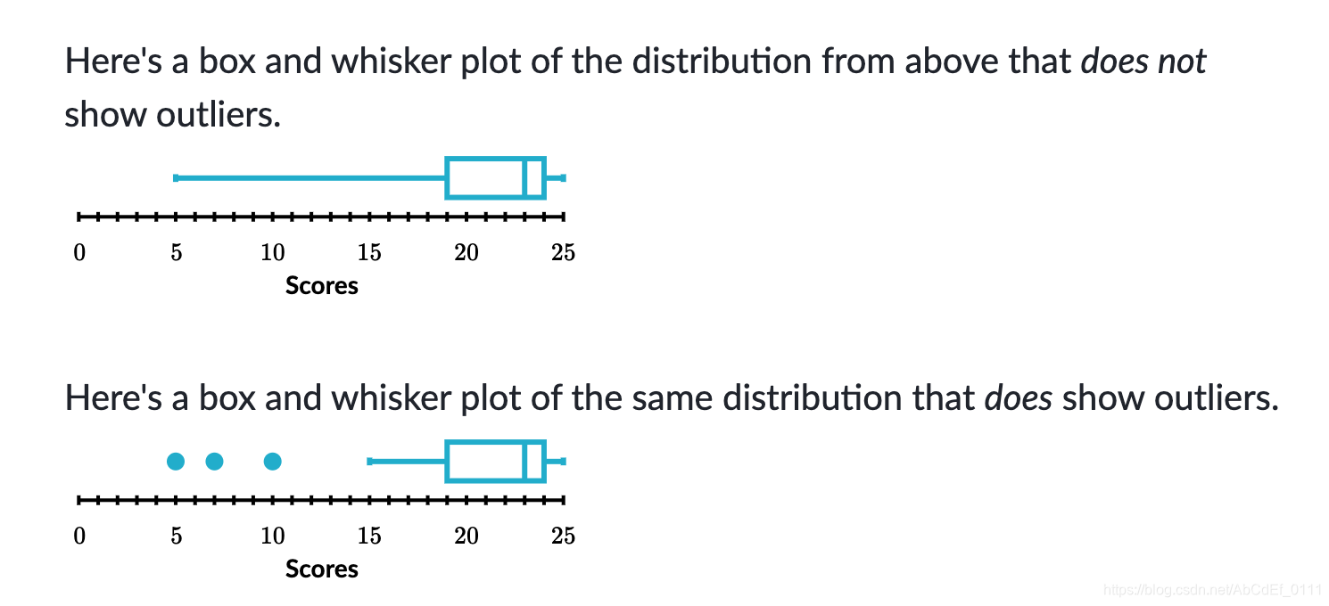
In this example, the outliers are 5,7,10

Q1-1.5*IQR=11.5
Q3+1.5*IQR=31.5

PART 6 Other Measures of Spread

1. Range and mid-range

range = max-min
mid-range = (max+min)/2
Midrange is a statistical tool that identifies a measure of center like median, mean, or mode

2. Mean absolute deviation (MAD)

MAD = $\frac{\sum_{i=1}^N\left|x-u\right|}{N}$

MAD: on average, how far each data point is from the mean; the average distance of each data point from the mean
MAD gives us an idea about the variability in a dataset
The greater the MAD, the more spread out of the data from the mean

Khan Academy - Statistics and Probability - Unit 3 SUMMARIZING QUANTITIVE DATA

SUMMARIZING QUANTITIVE DATA

PART 1 Measuring center in quantitive data

PART 2 Interquartile range(IQR)

PART 3 Variance and standard deviation of population

PART 4 Variance and Standard Deviation of a Sample

PART 5 Box and Whisker Plots

PART 6 Other Measures of Spread

猜你喜欢