回归分析是统计学的核心问题,通常用来用一个或多个解释变量来预测相应变量,有效的回归是一个交互的、整体的、多步骤的过程,而不仅仅是一个技巧
OLS回归
为了能够恰当地解释OLS模型的系数,数据必须满足以下假设:
- 正态性,即对于固定的自变量值,因变量值呈正态分布
- 独立性,因变量值之间相互独立
- 线性, 因变量与自变量之间线性相关
- 同方差性,因变量的方差不随自变量的水平不同而变化
如果违背上述假设,统计检验结果或所得的置信区间很可能就不精确了
简单线性回归
- 数据准备
提取鸢尾花数据中的山鸢尾数据作为本次回归数据源,该数据前文已经介绍,可参考鸢尾花数据简介。
#import data
> setosa <- filter(iris,Species=="setosa")

#view the structure of data
> names(setosa)
[1] "Sepal.Length" "Sepal.Width"  "Petal.Length" "Petal.Width"  "Species"
> summary(setosa)
  Sepal.Length    Sepal.Width     Petal.Length    Petal.Width          Species
 Min.   :4.300   Min.   :2.300   Min.   :1.000   Min.   :0.100   setosa    :50
 1st Qu.:4.800   1st Qu.:3.200   1st Qu.:1.400   1st Qu.:0.200   versicolor: 0
 Median :5.000   Median :3.400   Median :1.500   Median :0.200   virginica : 0
 Mean   :5.006   Mean   :3.428   Mean   :1.462   Mean   :0.246
 3rd Qu.:5.200   3rd Qu.:3.675   3rd Qu.:1.575   3rd Qu.:0.300
 Max.   :5.800   Max.   :4.400   Max.   :1.900   Max.   :0.600
> head(setosa)
  Sepal.Length Sepal.Width Petal.Length Petal.Width Species
1          5.1         3.5          1.4         0.2  setosa
2          4.9         3.0          1.4         0.2  setosa
3          4.7         3.2          1.3         0.2  setosa
4          4.6         3.1          1.5         0.2  setosa
5          5.0         3.6          1.4         0.2  setosa
6          5.4         3.9          1.7         0.4  setosa
> str(setosa)
'data.frame':	50 obs. of  5 variables:
 $ Sepal.Length: num  5.1 4.9 4.7 4.6 5 5.4 4.6 5 4.4 4.9 ...
 $ Sepal.Width : num  3.5 3 3.2 3.1 3.6 3.9 3.4 3.4 2.9 3.1 ...
 $ Petal.Length: num  1.4 1.4 1.3 1.5 1.4 1.7 1.4 1.5 1.4 1.5 ...
 $ Petal.Width : num  0.2 0.2 0.2 0.2 0.2 0.4 0.3 0.2 0.2 0.1 ...
 $ Species     : Factor w/ 3 levels "setosa","versicolor",..: 1 1 1 1 1 1 1 1 1 1 ...
- 绘制变量间的二元关系图
#Draws a binary diagram between variables
library(car)
scatterplot(Sepal.Width~Sepal.Length,data = setosa,
            spread=FALSE,smoother.args=list(lty=2),pch=19,
            xlab = "Sepal.Length",
            ylab = "Sepal.Width",
            main="Setosa")
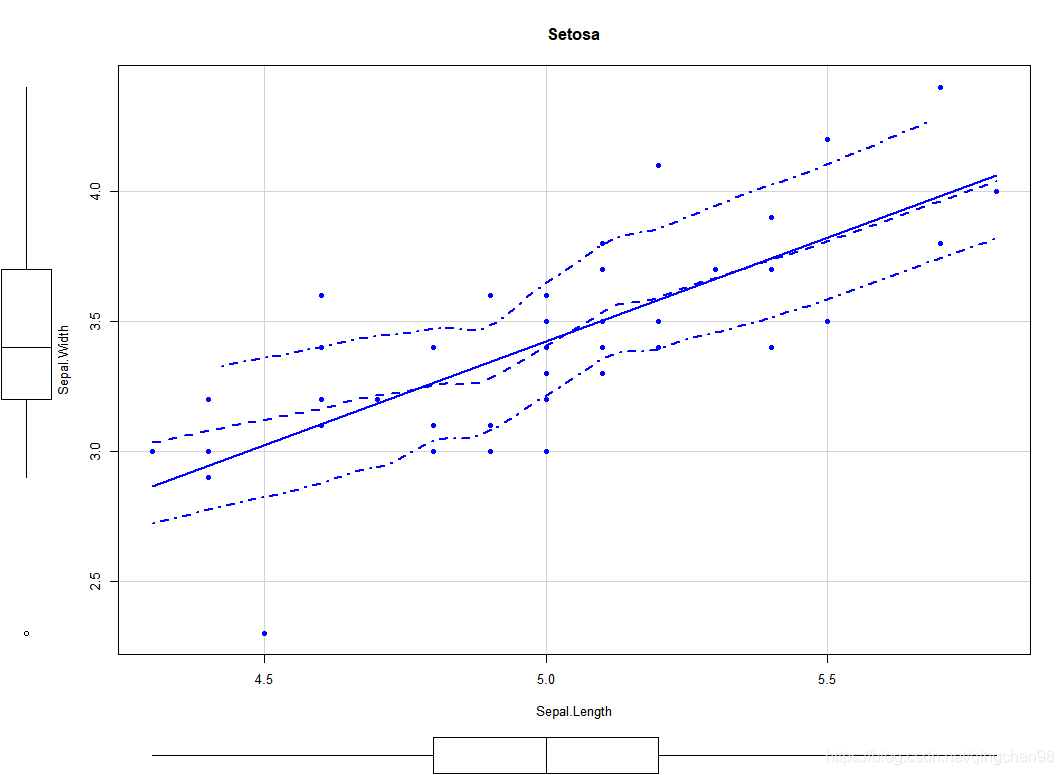
从图中可以看出,花萼的长度与宽度之间存在一定的线性关系,下一步建立模型进行分析。
- 建模分析
#creat a simple OLS model
> fit1 <- lm(Sepal.Width~Sepal.Length,data = setosa)
#reture the results of model
> summary(fit1)
Call:
lm(formula = Sepal.Width ~ Sepal.Length, data = setosa)
Residuals:
Min 1Q Median 3Q Max
-0.72394 -0.18273 -0.00306 0.15738 0.51709
Coefficients:
Estimate Std. Error t value Pr(>|t|)
(Intercept) -0.5694 0.5217 -1.091 0.281
Sepal.Length 0.7985 0.1040 7.681 6.71e-10 ***
---
Signif. codes: 0 ‘***’ 0.001 ‘**’ 0.01 ‘*’ 0.05 ‘.’ 0.1 ‘ ’ 1
Residual standard error: 0.2565 on 48 degrees of freedom
Multiple R-squared: 0.5514, Adjusted R-squared: 0.542
F-statistic: 58.99 on 1 and 48 DF, p-value: 6.71e-10
#return predicting value
> fitted(fit1)
1 2 3 4 5 6 7 8 9 10 11
3.503062 3.343356 3.183650 3.103798 3.423209 3.742620 3.103798 3.423209 2.944092 3.343356 3.742620
12 13 14 15 16 17 18 19 20 21 22
3.263503 3.263503 2.864239 4.062031 3.982179 3.742620 3.503062 3.982179 3.503062 3.742620 3.503062
23 24 25 26 27 28 29 30 31 32 33
3.103798 3.503062 3.263503 3.423209 3.423209 3.582914 3.582914 3.183650 3.263503 3.742620 3.582914
34 35 36 37 38 39 40 41 42 43 44
3.822473 3.343356 3.423209 3.822473 3.343356 2.944092 3.503062 3.423209 3.023945 2.944092 3.423209
45 46 47 48 49 50
3.503062 3.263503 3.503062 3.103798 3.662767 3.423209
#return residuals
> residuals(fit1)
1 2 3 4 5 6 7 8
-0.00306166 -0.34335600 0.01634966 -0.00379751 0.17679117 0.15737985 0.29620249 -0.02320883
9 10 11 12 13 14 15 16
-0.04409185 -0.24335600 -0.04262015 0.13649683 -0.26350317 0.13576098 -0.06203147 0.41782136
17 18 19 20 21 22 23 24
0.15737985 -0.00306166 -0.18217864 0.29693834 -0.34262015 0.19693834 0.49620249 -0.20306166
25 26 27 28 29 30 31 32
0.13649683 -0.42320883 -0.02320883 -0.08291449 -0.18291449 0.01634966 -0.16350317 -0.34262015
33 34 35 36 37 38 39 40
0.51708551 0.37752702 -0.24335600 -0.22320883 -0.32247298 0.25664400 0.05590815 -0.10306166
41 42 43 44 45 46 47 48
0.07679117 -0.72394468 0.25590815 0.07679117 0.29693834 -0.26350317 0.29693834 0.09620249
49 50
0.03723268 -0.12320883
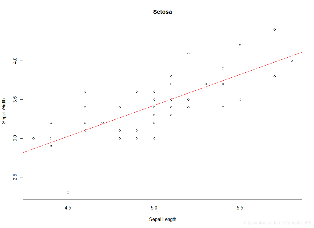
#plot the results
> plot(setosa$Sepal.Length,setosa$Sepal.Width,
+ xlab = "Sepal.Length",
+ ylab = "Sepal.Width",
+ main="Setosa")
> abline(fit1,col="red")
多项式回归
多项式回归只需在简单回归的基础上加点参数即可
> fit2 <- lm(Sepal.Width~Sepal.Length+I(Sepal.Length^2),data = setosa)
> summary(fit2)

Call:
lm(formula = Sepal.Width ~ Sepal.Length + I(Sepal.Length^2),
    data = setosa)

Residuals:
    Min      1Q  Median      3Q     Max
-0.7429 -0.1845  0.0112  0.1552  0.5283

Coefficients:
                  Estimate Std. Error t value Pr(>|t|)
(Intercept)         2.5020     5.9163   0.423    0.674
Sepal.Length       -0.4295     2.3586  -0.182    0.856
I(Sepal.Length^2)   0.1222     0.2344   0.521    0.605

Residual standard error: 0.2585 on 47 degrees of freedom
Multiple R-squared:  0.554,	Adjusted R-squared:  0.535
F-statistic: 29.19 on 2 and 47 DF,  p-value: 5.76e-09
可以发现,该数据集利用多项式回归预测效果不明显
多元线性回归
本次用到的数据集为state.x77,是美国50个州的统计数据,用该数据集来探究一个州的犯罪率与其他因素的关系,首先看一下数据集介绍:
- state.x77:
matrix with 50 rows and 8 columns giving the following statistics in the respective columns. - Population:
population estimate as of July 1, 1975 - Income:
per capita income (1974) - Illiteracy:
illiteracy (1970, percent of population) - Life Exp:
life expectancy in years (1969–71) - Murder:
murder and non-negligent manslaughter rate per 100,000 population (1976) - HS Grad:
percent high-school graduates (1970) - Frost:
mean number of days with minimum temperature below freezing (1931–1960) in capital or large city - Area:
land area in square miles - 数据准备
#extract data
There were 50 or more warnings (use warnings() to see the first 50)
> states_data <- as.data.frame(state.x77[,c("Murder","Population","Illiteracy",
+ "Income","Frost")])
> #the correlation index
> cor(states_data)
Murder Population Illiteracy Income Frost
Murder 1.0000000 0.3436428 0.7029752 -0.2300776 -0.5388834
Population 0.3436428 1.0000000 0.1076224 0.2082276 -0.3321525
Illiteracy 0.7029752 0.1076224 1.0000000 -0.4370752 -0.6719470
Income -0.2300776 0.2082276 -0.4370752 1.0000000 0.2262822
Frost -0.5388834 -0.3321525 -0.6719470 0.2262822 1.0000000
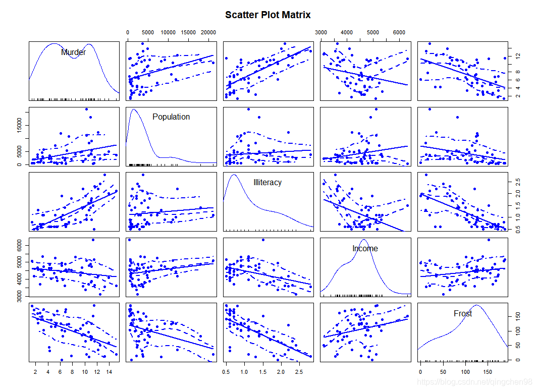
> #view the relationship between variables
> library(car)
> scatterplotMatrix(states_data,spread=FALSE,
+ smoother.args=list(lty=2),pch=19,
+ main="Scatter Plot Matrix")
There were 50 or more warnings (use warnings() to see the first 50)
- 建立多项式模型
 #creat a model
> fit3 <- lm(Murder~Population+Illiteracy+Income+Frost,data = states_data)
> summary(fit3)

Call:
lm(formula = Murder ~ Population + Illiteracy + Income + Frost,
    data = states_data)

Residuals:
    Min      1Q  Median      3Q     Max
-4.7960 -1.6495 -0.0811  1.4815  7.6210

Coefficients:
             Estimate Std. Error t value Pr(>|t|)
(Intercept) 1.235e+00  3.866e+00   0.319   0.7510
Population  2.237e-04  9.052e-05   2.471   0.0173 *
Illiteracy  4.143e+00  8.744e-01   4.738 2.19e-05 ***
Income      6.442e-05  6.837e-04   0.094   0.9253
Frost       5.813e-04  1.005e-02   0.058   0.9541
---
Signif. codes:  0 ‘***’ 0.001 ‘**’ 0.01 ‘*’ 0.05 ‘.’ 0.1 ‘ ’ 1

Residual standard error: 2.535 on 45 degrees of freedom
Multiple R-squared:  0.567,	Adjusted R-squared:  0.5285
F-statistic: 14.73 on 4 and 45 DF,  p-value: 9.133e-08