本篇文章主要是介绍一个北京二手房数据分析的项目,目的是熟悉python数据分析的及可视化的一些常用方法。
数据获取
通过编写python脚本(爬虫)从二手房交易数据网站上获取北京二手房数据集
数据解释
Direction:方向
District:区域
Elevator:电梯
Floor:楼层
Garden;花园
Id:编号
Layout:布局
Price:价格
Region:地区
Renovation:翻修,革新
Size:大小
Year:年限
## python源代码
# 1.数据初探
# 1.1首先导入要使用的科学计算包numpy,pandas,可视化matplotlib,seaborn,以及机器学习包sklearn。
import pandas as pd
import numpy as np
import seaborn as sns
import matplotlib as mpl
import matplotlib.pyplot as plt
from IPython.display import display
plt.style.use("fivethirtyeight")
sns.set_style({'font.sans-serif': ['simhei', 'Arial']})
# % matplotlib inline
# 检查Python版本
from sys import version_info
if version_info.major != 3:
raise Exception('请使用Python 3 来完成此项目')
# 1.2然后导入数据,并进行初步的观察,这些观察包括了解数据特征的缺失值,异常值,以及大概的描述性统计。
# 导入链家二手房数据
lianjia_df = pd.read_csv('lianjia.csv')
display(lianjia_df.head(n=2))
# 检查缺失值情况
lianjia_df.info()
# 1.3初步观察到一共有11个特征变量,Price 在这里是我们的目标变量,然后我们继续深入观察一下。
# 检查缺失值情况
lianjia_df.info()
lianjia_df.describe()
# 添加新特征房屋均价
df = lianjia_df.copy()
df['PerPrice'] = lianjia_df['Price'] / lianjia_df['Size']
# 重新摆放列位置
columns = ['Region', 'District', 'Garden', 'Layout', 'Floor', 'Year', 'Size', 'Elevator', 'Direction', 'Renovation',
'PerPrice', 'Price']
df = pd.DataFrame(df, columns=columns)
# 重新审视数据集
display(df.head(n=2))
# 2 数据可视化分析
# 2.1 Region特征分析
# 对于区域特征,我们可以分析不同区域房价和数量的对比。
# 对二手房区域分组对比二手房数量和每平米房价
# 使用了pandas的网络透视功能 groupby 分组排序。
# 区域特征可视化直接采用 seaborn 完成,颜色使用调色板 palette 参数,颜色渐变,越浅说明越少,反之越多
df_house_count = df.groupby('Region')['Price'].count().sort_values(ascending=False).to_frame().reset_index()
df_house_mean = df.groupby('Region')['PerPrice'].mean().sort_values(ascending=False).to_frame().reset_index()
f, [ax1, ax2, ax3] = plt.subplots(3, 1, figsize=(20, 15))
sns.barplot(x='Region', y='PerPrice', palette="Blues_d", data=df_house_mean, ax=ax1)
ax1.set_title('北京各大区二手房每平米单价对比', fontsize=12)
ax1.set_xlabel('区域', fontsize=12)
ax1.set_ylabel('每平米单价', fontsize=12)
sns.barplot(x='Region', y='Price', palette="Greens_d", data=df_house_count, ax=ax2)
ax2.set_title('北京各大区二手房数量对比', fontsize=12)
ax2.set_xlabel('区域', fontsize=12)
ax2.set_ylabel('数量', fontsize=12)
sns.boxplot(x='Region', y='Price', data=df, ax=ax3)
ax3.set_title('北京各大区二手房房屋总价', fontsize=12)
ax3.set_xlabel('区域', fontsize=12)
ax3.set_ylabel('房屋总价', fontsize=12)
# plt.show()
plt.savefig("Region.png")
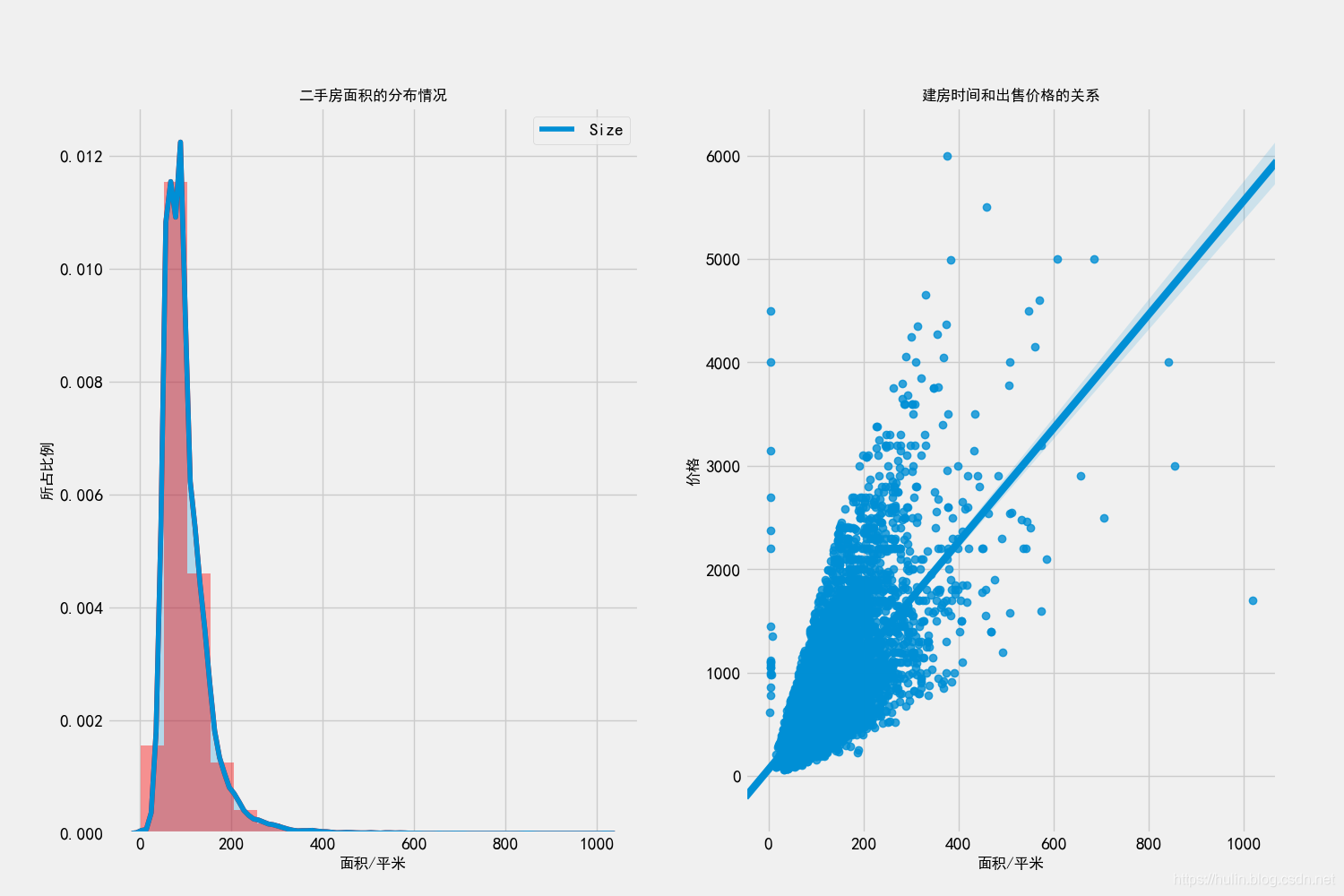
# 2.2 Size特征分析
f, [ax1, ax2] = plt.subplots(1, 2, figsize=(15, 10))
# 二手房面积的分布情况
sns.distplot(df['Size'], bins=20, ax=ax1, color='r')
sns.kdeplot(df['Size'], shade=True, ax=ax1)
ax1.set_title('二手房面积的分布情况', fontsize=12)
ax1.set_xlabel('面积/平米', fontsize=12)
ax1.set_ylabel('所占比例', fontsize=12)
# 建房时间和出售价格的关系
sns.regplot(x='Size', y='Price', data=df, ax=ax2)
ax2.set_title('建房时间和出售价格的关系', fontsize=12)
ax2.set_xlabel('面积/平米', fontsize=12)
ax2.set_ylabel('价格', fontsize=12)
# plt.show()
plt.savefig('Size.png')
print("房屋面积小于10平米:")
print(df.loc[df['Size'] < 10])
print("房屋面积大于1000平米:")
print(df.loc[df['Size'] > 1000])
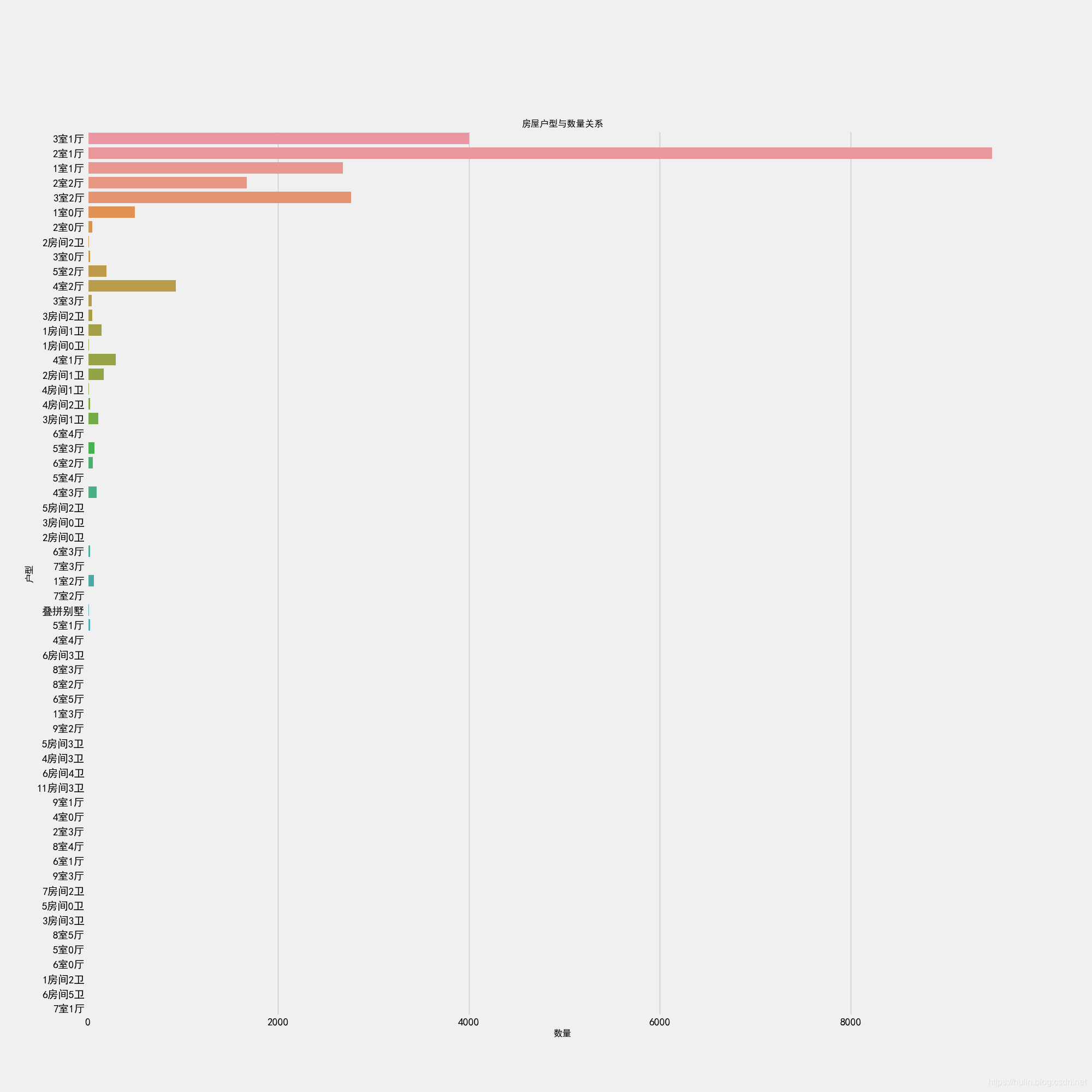
# 2.3 Layout特征分析
f, ax1 = plt.subplots(figsize=(20, 20))
sns.countplot(y='Layout', data=df, ax=ax1)
ax1.set_title('房屋户型与数量关系', fontsize=12)
ax1.set_xlabel('数量', fontsize=12)
ax1.set_ylabel('户型', fontsize=12)
# plt.show()
plt.savefig('Layout.png')
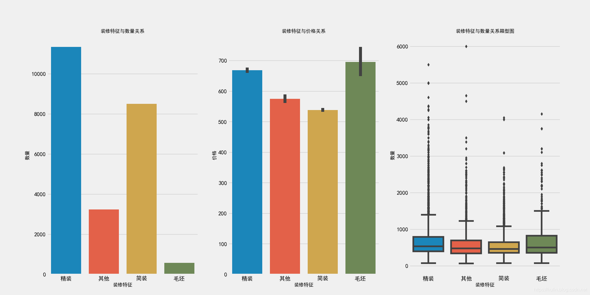
# 2.4Renovation特征分析
print(df['Renovation'].value_counts())
# 去掉数据中装修特征“南北”
df['Renovation'] = df.loc[(df['Renovation'] != '南北'), 'Renovation']
# 画幅设置
f, [ax1, ax2, ax3] = plt.subplots(1, 3, figsize=(20, 10))
sns.countplot(df['Renovation'], ax=ax1)
ax1.set_title('装修特征与数量关系', fontsize=12)
ax1.set_xlabel('装修特征', fontsize=12)
ax1.set_ylabel('数量', fontsize=12)
sns.barplot(x='Renovation', y='Price', data=df, ax=ax2)
ax2.set_title('装修特征与价格关系', fontsize=12)
ax2.set_xlabel('装修特征', fontsize=12)
ax2.set_ylabel('价格', fontsize=12)
sns.boxplot(x='Renovation', y='Price', data=df, ax=ax3)
ax3.set_title('装修特征与数量关系箱型图', fontsize=12)
ax3.set_xlabel('装修特征', fontsize=12)
ax3.set_ylabel('数量', fontsize=12)
# plt.show()
plt.savefig('Renovation.png')
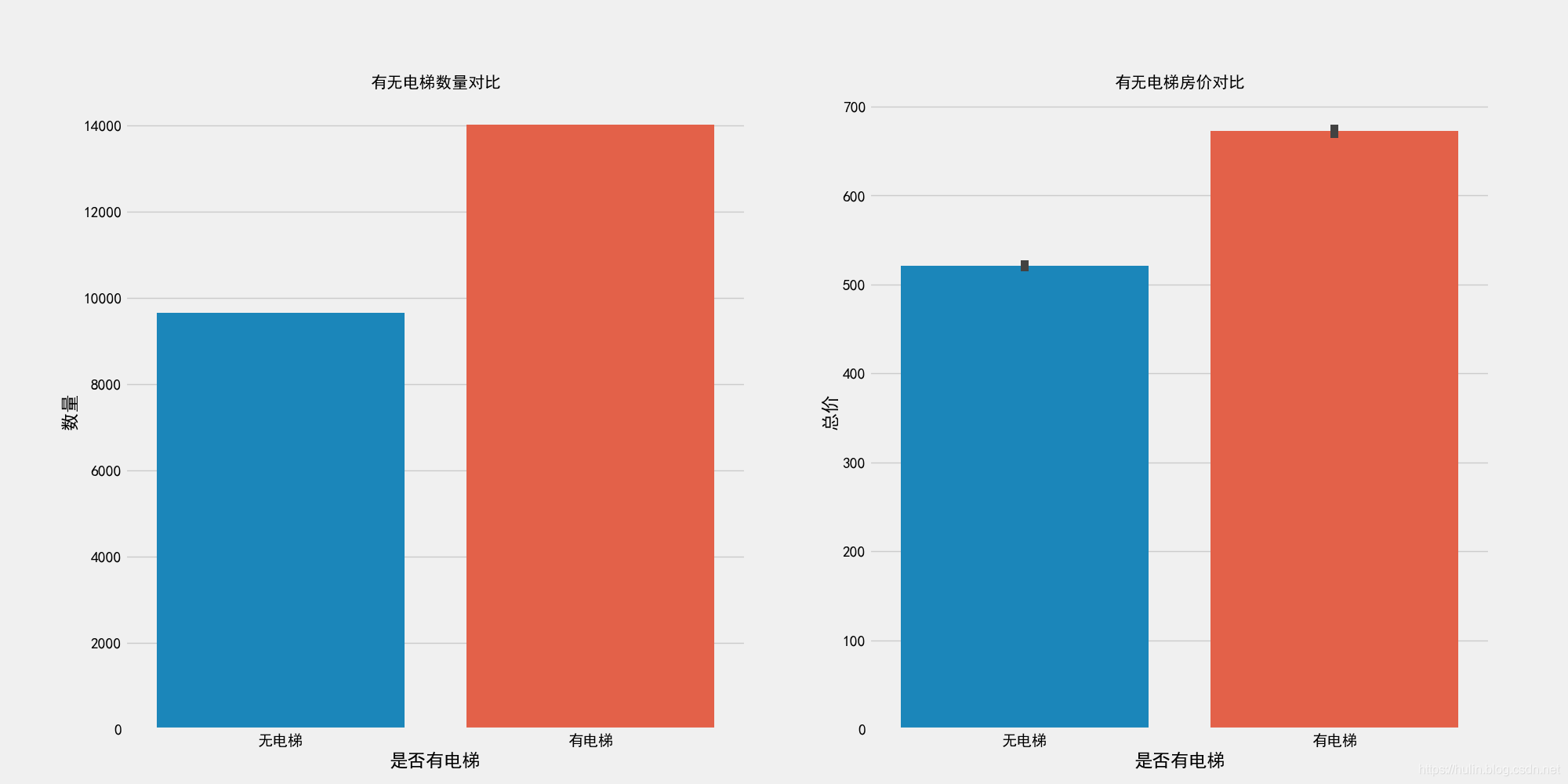
# 2.5Elevator特征分析
# 初探数据时,Elevator有大量的缺失值
misn = len(df.loc[(df['Elevator'].isnull()), 'Elevator'])
print("电梯的缺失值数量:", misn)
# 由于存在个别类型错误,如简装和精装,特征值错位,故需要移除
df['Elevator'] = df.loc[(df['Elevator'] == '有电梯') | (df['Elevator'] == '无电梯'), 'Elevator']
# 填补Elevator缺失值
df.loc[(df['Floor'] > 6) & (df['Elevator'].isnull()), 'Elevator'] = '有电梯'
df.loc[(df['Floor'] <= 6) & (df['Elevator'].isnull()), 'Elevator'] = '无电梯'
f, [ax1, ax2] = plt.subplots(1, 2, figsize=(20, 10))
sns.countplot(df['Elevator'], ax=ax1)
ax1.set_title('有无电梯数量对比', fontsize=15)
ax1.set_xlabel('是否有电梯')
ax1.set_ylabel('数量')
sns.barplot(x='Elevator', y='Price', data=df, ax=ax2)
ax2.set_title('有无电梯房价对比', fontsize=15)
ax2.set_xlabel('是否有电梯')
ax2.set_ylabel('总价')
# plt.show()
plt.savefig("Elevator.png")
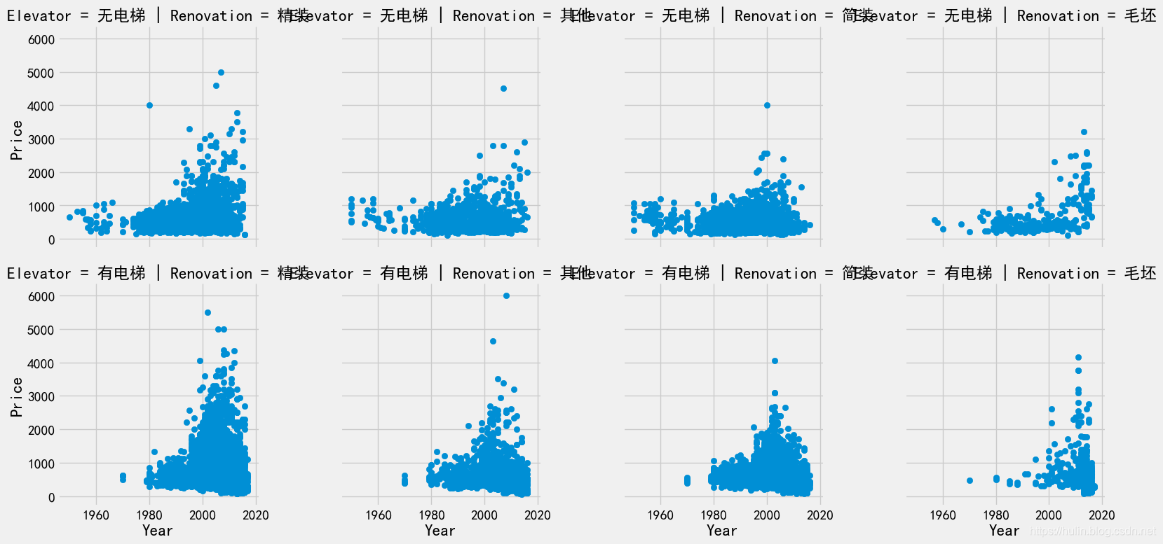
#2.6 Year特征分析
grid = sns.FacetGrid(df, row='Elevator', col='Renovation', palette='seismic',size=4)
grid.map(plt.scatter, 'Year', 'Price')
grid.add_legend()
grid.savefig("Year.png")
分析结果
二手房均价:西城区的房价最贵均价大约11万/平,因为西城在二环以里,且是热门学区房的聚集地。其次是东城大约10万/平,然后是海淀大约8.5万/平,其它均低于8万/平。
二手房房数量:从数量统计上来看,目前二手房市场上比较火热的区域。海淀区和朝阳区二手房数量最多,差不多都接近3000套,毕竟大区,需求量也大。然后是丰台区,近几年正在改造建设,有赶超之势。
二手房总价:通过箱型图看到,各大区域房屋总价中位数都都在1000万以下,且房屋总价离散值较高,西城最高达到了6000万,说明房屋价格特征不是理想的正太分布。
1.Region特征分析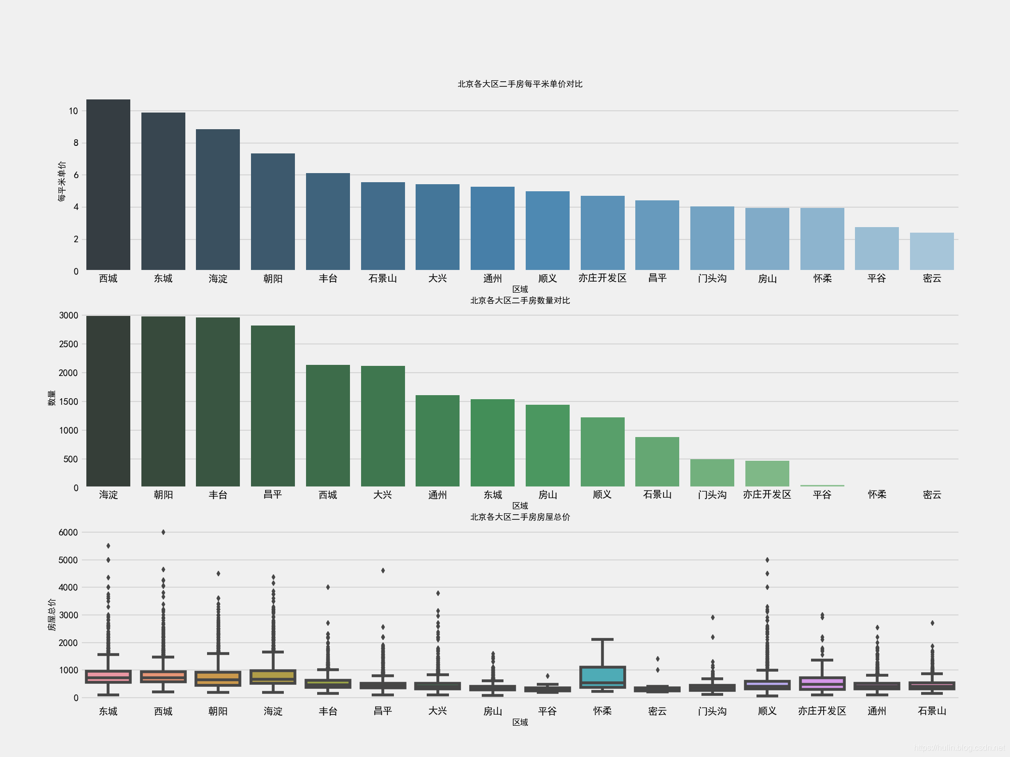
2.Size特征分析
3.Layout特征分析
4.Renovation特征分析
5.Elevator特征分析
6.Year特征分析