数学中的图像重构 -- CT中的 Radon 变换 图解

这是我之前在剑桥大学上的一节研究生应数选修课 Image Reconstruction，之前没怎么听懂，所以这段时间想把它补起来。
这节课老师没有明确的讲义，所以我就照记着的一些书的顺序，把它复习了。
整堂课只有我一个人上 QAQ，所以应该算是在数学系里比较小众的方向吧。
因此这篇笔记 基本上是为了 我自己以后查资料或公式好找一点。
笔记部分摘自 Mathematical Methods in Image Reconstruction. F.Natterer and F.Wuebbeling.

• 笔记总目录
• 专栏

引言

图像重构 Intro

Radon Transform 拉东变换 ${\color{red}\mathcal{R}f}$

• 拉东变换是一个积分变换

• 先它将定义在二维平面上的一个函数 $f(x_1,x_2)$ 沿着平面上的任意一条直线做线积分，相当于对函数 $f(x_1,x_2)$ 做 CT扫描

• 令 X射线 在 $x$ 点 线性衰减后 为 $f(x)$。 那么 X射线光束 $L$ 经过的部分成像就是 $g(L)=\int_L f(x)dx$ 。

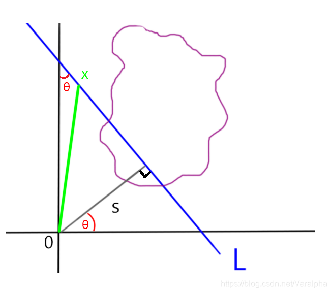
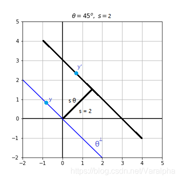
• 如果我们用 $s$ （原点到射线的距离）与 $\theta$ （距离的夹角）表示射线 $L$， 如图：

• 可得这条直线为 $L(\theta,s) = \{x\in \R^2: x\cdot \theta = s\},\; \theta \in S^1, \; s\in \R^1$

• 可得如下方程：

$g(\theta,s) = \int_{x\cdot \theta = s} f(x)dx = (\mathcal{R}f)(\theta,s)$

• 用python把它表示出来：

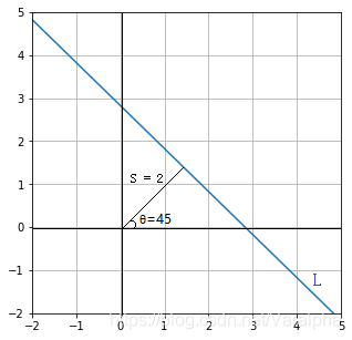
import matplotlib.pyplot as plt
import numpy as np
# 为了之后扩展到 n 维 这里用 x_1 x_2 表示  
x1 = np.arange(-10,10.01,.01) # x_1 可以理解为 二维(x,y) 坐标轴的x
x2 = np.arange(-10,10.01,.01) # x_2 可以理解为 二维(x,y) 坐标轴的y
xv = np.meshgrid(x1,x2) # 网格化
degree = 45 # theta 角度  
theta = degree/180 *np.pi
s = 2. # s 长度
Lv = abs(xv[0]*np.cos(theta) + xv[1]*np.sin(theta)-s) # x1*cos(theta) + x2*cos(theta) - s = 0
L = np.max((Lv<0.01)*xv[1],axis=0)+np.min((Lv<0.01)*xv[1],axis=0) # 筛选出 满足条件的值
# L.nonzero()  L 的非零值坐标  
plt.plot(x1[L.nonzero()],L[L.nonzero()],'blue')
plt.show()

• 我还做了变量为 $s$ 和 $\theta$ 的动图：

• 接下来，把它拓展到更高维度 n 维。
• 构筑 n 维超平面 $H(\theta,s) = \{x\in \R^n: x\cdot \theta = s\},\; \theta \in S^{n-1} \text{ (unit sphere) }, \; s\in \R^1$
• 超平面垂直于 $\theta$ 距离为 $s$
• 同时 $H(-\theta,-s) = H(\theta,s)$ 为 偶函数
• 可定义

$(\mathcal{R}f) (\theta, s)= \int_{x\cdot \theta = s} f(x)dx = \int_{H(\theta,s)}f(x) dx$

• $\mathcal{R}f$ 函数在 单位圆柱 unit sylinder 上

${\color{red}C^n} = \{(\theta,s): \theta \in S^{n-1} ,\; s\in \R^1\}$

• 因为 $H(-\theta,-s) = H(\theta,s)$ ， 所以 $(\mathcal{R}f)(-\theta,-s) = \mathcal{R}f(\theta,s)$ 为偶函数

• 由于 $s - x\cdot \theta = 0$ 变换可得：

$(\mathcal{R}f)(\theta,s) = \int_{\R^n} \delta(s - x \cdot \theta) f(x) dx$

• $\theta^\perp = \{x\in\R^n: x\cdot \theta = 0\}$ 正交 $\theta$ 的子空间

$(\mathcal{R}f)(\theta,s) = \int_{\theta^\perp}f(s\theta + y) dy$

• 由于 $f \in {\color{red}\mathcal{S}(\R^n)}$ 在速降函数空间内（Schwartz space）
• 那么 $\mathcal{R}f \in \mathcal{S}(C^n)$
• ${\color{red}\mathcal{S}(C^n)}$ 为

$\mathcal{S}(C^n) = \Big \{ g \in \mathcal{C}^\infty(C^n): s^l \frac{\partial^k}{\partial s^k} g(\theta,s) \text{ bounded }, \; l,k = 0,1,\cdots \Big \}$

• ${\color{red}\mathcal{C}^\infty}(C^n)$ 是所有从 $C^n$ 射到 $\mathcal{C}$ 的光滑函数 (无穷阶可导的函数)

• 卷积运算

$(g \star h)(\theta, s) = \int_{\R^1} g(\theta, s-t)h(\theta, t)dt$

傅里叶变换 ${\color{red}\mathcal{F}}$

$\mathcal{F}(g(\theta, s)) = (2\pi)^{-1/2} \int_{\R^1}g(\theta, s) e^{-is\sigma} ds$

• 当 $f\in \mathcal{S}(\R^n), \; \theta \in S^{n-1} \text{ (unit sphere) }, \; \sigma \in \R^1$

$\mathcal{F}\big[(\mathcal{R}f)(\theta, \sigma)\big]_{C^n} = (2\pi)^{\frac{n-1}{2}}\mathcal{F}[f(\sigma \theta)]_{\R^n}$

• 当 $f, g \in \mathcal{S}(\R^n)$

$\underset{C^n}{\mathcal{R}f \star \mathcal{R}g} = \underset{\R^n}{\mathcal{R}(f\star g)}$

BackProjection operator 后向投影 算子 ${\color{red}\mathcal{R}^*}$

$(\mathcal{R}^* g)(x) = \int_{S^{n-1}} g(\theta, x\cdot \theta) d\theta, \; g\in \mathcal{S}(C^n)$

• 因此 对于 $g = \mathcal{R}f, \; (\mathcal{R}^*g)(x)$ 是 所有超平面 经过 $x$, $f$ 的积分 的均值。

• 在数学中 可以说 $\mathcal{R}^*$ 是 $\mathcal{R}$ 的共轭

• 对于 $g \in \mathcal{S}(\R^1), \; f\in \mathcal{S}(\R^n)$

$\int_{\R^1} g(s) (\mathcal{R}f)(\theta,s) ds = \int_{\R^n} g(x \cdot \theta)f(x) dx$

• 对于 $g \in \mathcal{S}(C^n), \; f\in \mathcal{S}(\R^n)$

$\int_{S^{n-1}}\int_{\R^1} g \mathcal{R}f d\theta ds = \int_{\R^n} (\mathcal{R}^*g)f(x)d(x) dx$

• 当 $f\in \mathcal{S}(\R^n)$ 和 $g\in \mathcal{S}(C^n)$

$(\mathcal{R}^*g ) \star f = \mathcal{R}^* (g \star \mathcal{R}f)$

• 当 $g\in\mathcal{S}(C^n)$ 为偶 (例 $g(\theta,s)= g(-\theta,-s)$ )

$\mathcal{F}\big[(\mathcal{R}^* g)(\xi)\big] = 2 (2\pi)^{\frac{n-1}{2}}\lvert \xi \rvert^{1-n} \mathcal{F}\Big[g(\frac{\xi}{\lvert \xi \rvert},\lvert \xi \rvert)\Big]$

• 通过 Riesz potential 里斯位势 在 $C^n$

$\mathcal{F}\big[(\mathcal{I}^\alpha g)(\theta, \sigma)\big] = \lvert \sigma \rvert^{-\alpha} \mathcal{F}\Big[g(\theta,\sigma)\Big], \; \alpha <1$